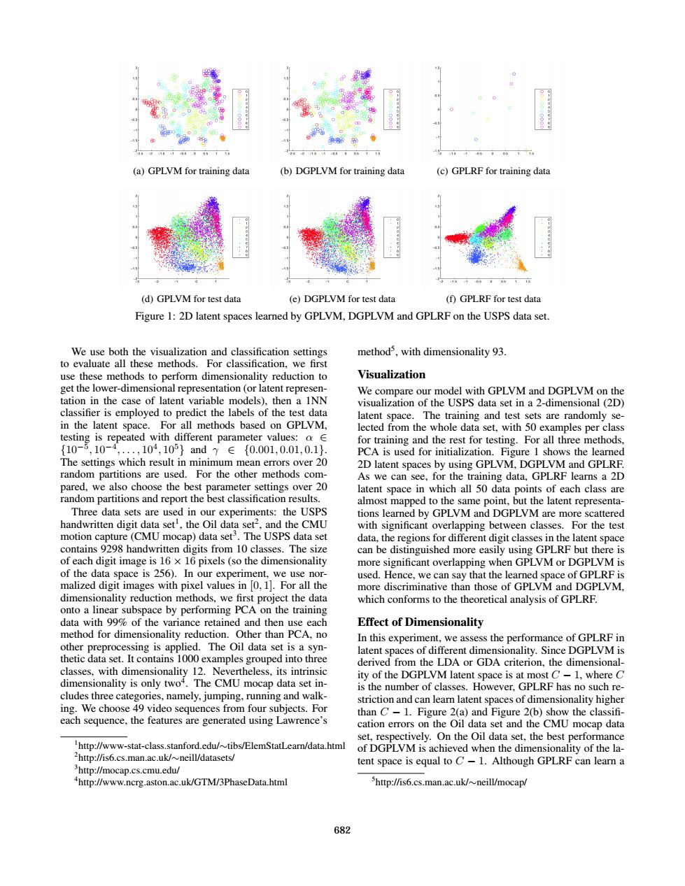
11 (a)GPLVM for training data (b)DGPLVM for training data (c)GPLRF for training data (d)GPLVM for test data (e)DGPLVM for test data (f)GPLRF for test data Figure 1:2D latent spaces learned by GPLVM,DGPLVM and GPLRF on the USPS data set. We use both the visualization and classification settings method3,with dimensionality 93. to evaluate all these methods.For classification.we first use these methods to perform dimensionality reduction to Visualization get the lower-dimensional representation (or latent represen- We compare our model with GPLVM and DGPLVM on the tation in the case of latent variable models),then a INN visualization of the USPS data set in a 2-dimensional(2D) classifier is employed to predict the labels of the test data latent space.The training and test sets are randomly se- in the latent space.For all methods based on GPLVM, lected from the whole data set,with 50 examples per class testing is repeated with different parameter values:o E for training and the rest for testing.For all three methods, {10-5,10-4,.,104,105}andy∈{0.001,0.01,0.1}. PCA is used for initialization.Figure 1 shows the learned The settings which result in minimum mean errors over 20 2D latent spaces by using GPLVM,DGPLVM and GPLRF. random partitions are used.For the other methods com- As we can see,for the training data,GPLRF learns a 2D pared,we also choose the best parameter settings over 20 latent space in which all 50 data points of each class are random partitions and report the best classification results. almost mapped to the same point,but the latent representa- Three data sets are used in our experiments:the USPS tions learned by GPLVM and DGPLVM are more scattered handwritten digit data set',the Oil data set2,and the CMU with significant overlapping between classes.For the test motion capture(CMU mocap)data set3.The USPS data set data,the regions for different digit classes in the latent space contains 9298 handwritten digits from 10 classes.The size can be distinguished more easily using GPLRF but there is of each digit image is 16 x 16 pixels(so the dimensionality more significant overlapping when GPLVM or DGPLVM is of the data space is 256).In our experiment,we use nor- used.Hence,we can say that the learned space of GPLRF is malized digit images with pixel values in [0,1].For all the more discriminative than those of GPLVM and DGPLVM. dimensionality reduction methods,we first project the data which conforms to the theoretical analysis of GPLRF. onto a linear subspace by performing PCA on the training data with 99%of the variance retained and then use each Effect of Dimensionality method for dimensionality reduction.Other than PCA.no In this experiment,we assess the performance of GPLRF in other preprocessing is applied.The Oil data set is a syn- latent spaces of different dimensionality.Since DGPLVM is thetic data set.It contains 1000 examples grouped into three derived from the LDA or GDA criterion,the dimensional- classes,with dimensionality 12.Nevertheless,its intrinsic ity of the DGPLVM latent space is at most C-1,where C dimensionality is only twoi.The CMU mocap data set in- is the number of classes.However,GPLRF has no such re- cludes three categories,namely,jumping,running and walk- striction and can learn latent spaces of dimensionality higher ing.We choose 49 video sequences from four subjects.For than C-1.Figure 2(a)and Figure 2(b)show the classifi- each sequence,the features are generated using Lawrence's cation errors on the Oil data set and the CMU mocap data set,respectively.On the Oil data set,the best performance http://www-stat-class.stanford.edu/tibs/ElemStatLearn/data.html of DGPLVM is achieved when the dimensionality of the la- http://is6.cs.man.ac.uk/neill/datasets/ tent space is equal to C-1.Although GPLRF can learn a http://mocap.cs.cmu.edu/ "http://www.ncrg.aston.ac.uk/GTM/3PhaseData.html http://is6.cs.man.ac.uk/~neill/mocap/ 682(a) GPLVM for training data (b) DGPLVM for training data (c) GPLRF for training data (d) GPLVM for test data (e) DGPLVM for test data (f) GPLRF for test data Figure 1: 2D latent spaces learned by GPLVM, DGPLVM and GPLRF on the USPS data set. We use both the visualization and classification settings to evaluate all these methods. For classification, we first use these methods to perform dimensionality reduction to get the lower-dimensional representation (or latent represen￾tation in the case of latent variable models), then a 1NN classifier is employed to predict the labels of the test data in the latent space. For all methods based on GPLVM, testing is repeated with different parameter values: α ∈ {10−5 , 10−4 , . . . , 104 , 105} and γ ∈ {0.001, 0.01, 0.1}. The settings which result in minimum mean errors over 20 random partitions are used. For the other methods com￾pared, we also choose the best parameter settings over 20 random partitions and report the best classification results. Three data sets are used in our experiments: the USPS handwritten digit data set1 , the Oil data set2 , and the CMU motion capture (CMU mocap) data set3 . The USPS data set contains 9298 handwritten digits from 10 classes. The size of each digit image is 16 × 16 pixels (so the dimensionality of the data space is 256). In our experiment, we use nor￾malized digit images with pixel values in [0, 1]. For all the dimensionality reduction methods, we first project the data onto a linear subspace by performing PCA on the training data with 99% of the variance retained and then use each method for dimensionality reduction. Other than PCA, no other preprocessing is applied. The Oil data set is a syn￾thetic data set. It contains 1000 examples grouped into three classes, with dimensionality 12. Nevertheless, its intrinsic dimensionality is only two4 . The CMU mocap data set in￾cludes three categories, namely, jumping, running and walk￾ing. We choose 49 video sequences from four subjects. For each sequence, the features are generated using Lawrence’s 1 http://www-stat-class.stanford.edu/∼tibs/ElemStatLearn/data.html 2 http://is6.cs.man.ac.uk/∼neill/datasets/ 3 http://mocap.cs.cmu.edu/ 4 http://www.ncrg.aston.ac.uk/GTM/3PhaseData.html method5 , with dimensionality 93. Visualization We compare our model with GPLVM and DGPLVM on the visualization of the USPS data set in a 2-dimensional (2D) latent space. The training and test sets are randomly se￾lected from the whole data set, with 50 examples per class for training and the rest for testing. For all three methods, PCA is used for initialization. Figure 1 shows the learned 2D latent spaces by using GPLVM, DGPLVM and GPLRF. As we can see, for the training data, GPLRF learns a 2D latent space in which all 50 data points of each class are almost mapped to the same point, but the latent representa￾tions learned by GPLVM and DGPLVM are more scattered with significant overlapping between classes. For the test data, the regions for different digit classes in the latent space can be distinguished more easily using GPLRF but there is more significant overlapping when GPLVM or DGPLVM is used. Hence, we can say that the learned space of GPLRF is more discriminative than those of GPLVM and DGPLVM, which conforms to the theoretical analysis of GPLRF. Effect of Dimensionality In this experiment, we assess the performance of GPLRF in latent spaces of different dimensionality. Since DGPLVM is derived from the LDA or GDA criterion, the dimensional￾ity of the DGPLVM latent space is at most C − 1, where C is the number of classes. However, GPLRF has no such re￾striction and can learn latent spaces of dimensionality higher than C − 1. Figure 2(a) and Figure 2(b) show the classifi- cation errors on the Oil data set and the CMU mocap data set, respectively. On the Oil data set, the best performance of DGPLVM is achieved when the dimensionality of the la￾tent space is equal to C − 1. Although GPLRF can learn a 5 http://is6.cs.man.ac.uk/∼neill/mocap/ 682