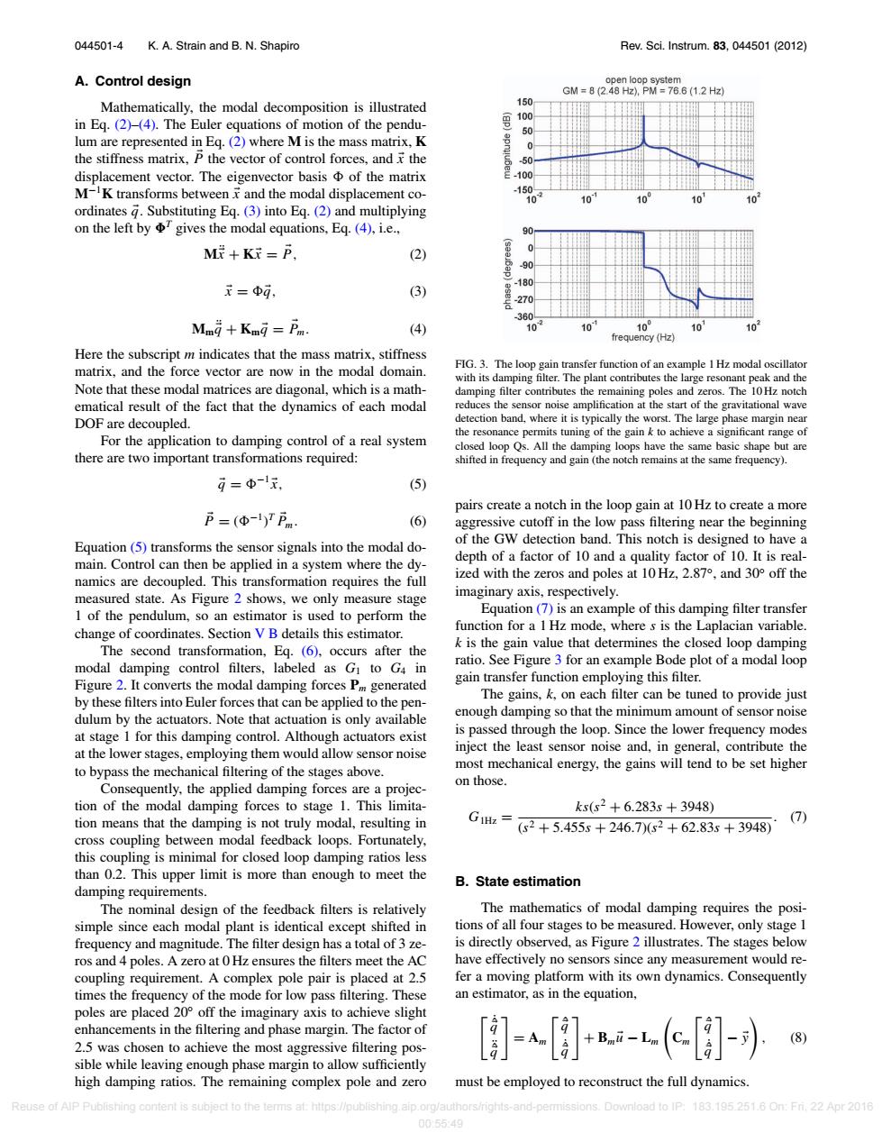
044501-4 K.A.Strain and B.N.Shapiro Rev.Sci.Instrum.83,044501 (2012) A.Control design open loop system GM=8(2.48Hz),PM=76.6(1.2Hz) Mathematically,the modal decomposition is illustrated 150 100 in Eq.(2)-(4).The Euler equations of motion of the pendu- 50 lum are represented in Eq.(2)where M is the mass matrix,K 0 the stiffness matrix,P the vector of control forces,and the -50 displacement vector.The eigenvector basis of the matrix -100 M-K transforms between and the modal displacement co- -15 0 10 10 10 10 ordinates g.Substituting Eq.(3)into Eq.(2)and multiplying on the left by gives the modal equations,Eq.(4),i.e., M+K=P, (2) 90 -180 元=Φd, (3) -270 -360 Mmg +Kmg Pm (4) 10 10 100 10 10 frequency (Hz) Here the subscript m indicates that the mass matrix,stiffness matrix.and the force vector are now in the modal domain. FIG.3.The loop gain transfer function of an example 1Hz modal oscillator with its damping filter.The plant contributes the large resonant peak and the Note that these modal matrices are diagonal,which is a math- damping filter contributes the remaining poles and zeros.The 10 Hz notch ematical result of the fact that the dynamics of each modal reduces the sensor noise amplification at the start of the gravitational wave DOF are decoupled. detection band,where it is typically the worst.The large phase margin near the resonance permits tuning of the gain k to achieve a significant range of For the application to damping control of a real system closed loop Qs.All the damping loops have the same basic shape but are there are two important transformations required: shifted in frequency and gain (the notch remains at the same frequency). g=Φ-1x, (5) pairs create a notch in the loop gain at 10 Hz to create a more P=(Φ-)TPm. (6) aggressive cutoff in the low pass filtering near the beginning of the GW detection band.This notch is designed to have a Equation (5)transforms the sensor signals into the modal do- main.Control can then be applied in a system where the dy- depth of a factor of 10 and a quality factor of 10.It is real- namics are decoupled.This transformation requires the full ized with the zeros and poles at10Hz,2.87°，and30°off the measured state.As Figure 2 shows,we only measure stage imaginary axis,respectively. 1 of the pendulum,so an estimator is used to perform the Equation(7)is an example of this damping filter transfer change of coordinates.Section V B details this estimator. function for a I Hz mode,where s is the Laplacian variable. k is the gain value that determines the closed loop damping The second transformation,Eg.(6),occurs after the modal damping control filters,labeled as G to G4 in ratio.See Figure 3 for an example Bode plot of a modal loop Figure 2.It converts the modal damping forces Pm generated gain transfer function employing this filter. by these filters into Euler forces that can be applied to the pen- The gains,k,on each filter can be tuned to provide just dulum by the actuators.Note that actuation is only available enough damping so that the minimum amount of sensor noise at stage 1 for this damping control.Although actuators exist is passed through the loop.Since the lower frequency modes at the lower stages,employing them would allow sensor noise inject the least sensor noise and,in general,contribute the to bypass the mechanical filtering of the stages above. most mechanical energy,the gains will tend to be set higher on those. Consequently,the applied damping forces are a projec- tion of the modal damping forces to stage 1.This limita- ks(s2+6.283s+3948) tion means that the damping is not truly modal,resulting in GIHz= (7) (s2+5.455s+246.7)(s2+62.83s+3948) cross coupling between modal feedback loops.Fortunately, this coupling is minimal for closed loop damping ratios less than 0.2.This upper limit is more than enough to meet the B.State estimation damping requirements. The nominal design of the feedback filters is relatively The mathematics of modal damping requires the posi- simple since each modal plant is identical except shifted in tions of all four stages to be measured.However,only stage 1 frequency and magnitude.The filter design has a total of 3 ze- is directly observed,as Figure 2 illustrates.The stages below ros and 4 poles.A zero at 0 Hz ensures the filters meet the AC have effectively no sensors since any measurement would re- coupling requirement.A complex pole pair is placed at 2.5 fer a moving platform with its own dynamics.Consequently times the frequency of the mode for low pass filtering.These an estimator,as in the equation, poles are placed 20 off the imaginary axis to achieve slight enhancements in the filtering and phase margin.The factor of 2.5 was chosen to achieve the most aggressive filtering pos- B.i-I sible while leaving enough phase margin to allow sufficiently high damping ratios.The remaining complex pole and zero must be employed to reconstruct the full dynamics Reuse of AlP Publishing content is subject to the terms at:https://publishing.aip.org/authors/nghts-and-perm Download to IP: 183.195251.60Fi.22Apr2016 00:5549044501-4 K. A. Strain and B. N. Shapiro Rev. Sci. Instrum. 83, 044501 (2012) A. Control design Mathematically, the modal decomposition is illustrated in Eq. (2)–(4). The Euler equations of motion of the pendu￾lum are represented in Eq. (2) where M is the mass matrix, K the stiffness matrix, P the vector of control forces, and x the displacement vector. The eigenvector basis of the matrix M−1K transforms between x and the modal displacement co￾ordinates q. Substituting Eq. (3) into Eq. (2) and multiplying on the left by T gives the modal equations, Eq. (4), i.e., M¨ x + Kx = P, (2) x = q, (3) Mm ¨ q + Kmq = P m. (4) Here the subscript m indicates that the mass matrix, stiffness matrix, and the force vector are now in the modal domain. Note that these modal matrices are diagonal, which is a math￾ematical result of the fact that the dynamics of each modal DOF are decoupled. For the application to damping control of a real system there are two important transformations required: q = −1x, (5) P = (−1 ) T P m. (6) Equation (5) transforms the sensor signals into the modal do￾main. Control can then be applied in a system where the dy￾namics are decoupled. This transformation requires the full measured state. As Figure 2 shows, we only measure stage 1 of the pendulum, so an estimator is used to perform the change of coordinates. Section V B details this estimator. The second transformation, Eq. (6), occurs after the modal damping control filters, labeled as G1 to G4 in Figure 2. It converts the modal damping forces Pm generated by these filters into Euler forces that can be applied to the pen￾dulum by the actuators. Note that actuation is only available at stage 1 for this damping control. Although actuators exist at the lower stages, employing them would allow sensor noise to bypass the mechanical filtering of the stages above. Consequently, the applied damping forces are a projec￾tion of the modal damping forces to stage 1. This limita￾tion means that the damping is not truly modal, resulting in cross coupling between modal feedback loops. Fortunately, this coupling is minimal for closed loop damping ratios less than 0.2. This upper limit is more than enough to meet the damping requirements. The nominal design of the feedback filters is relatively simple since each modal plant is identical except shifted in frequency and magnitude. The filter design has a total of 3 ze￾ros and 4 poles. A zero at 0 Hz ensures the filters meet the AC coupling requirement. A complex pole pair is placed at 2.5 times the frequency of the mode for low pass filtering. These poles are placed 20◦ off the imaginary axis to achieve slight enhancements in the filtering and phase margin. The factor of 2.5 was chosen to achieve the most aggressive filtering pos￾sible while leaving enough phase margin to allow sufficiently high damping ratios. The remaining complex pole and zero FIG. 3. The loop gain transfer function of an example 1 Hz modal oscillator with its damping filter. The plant contributes the large resonant peak and the damping filter contributes the remaining poles and zeros. The 10 Hz notch reduces the sensor noise amplification at the start of the gravitational wave detection band, where it is typically the worst. The large phase margin near the resonance permits tuning of the gain k to achieve a significant range of closed loop Qs. All the damping loops have the same basic shape but are shifted in frequency and gain (the notch remains at the same frequency). pairs create a notch in the loop gain at 10 Hz to create a more aggressive cutoff in the low pass filtering near the beginning of the GW detection band. This notch is designed to have a depth of a factor of 10 and a quality factor of 10. It is real￾ized with the zeros and poles at 10 Hz, 2.87◦, and 30◦ off the imaginary axis, respectively. Equation (7) is an example of this damping filter transfer function for a 1 Hz mode, where s is the Laplacian variable. k is the gain value that determines the closed loop damping ratio. See Figure 3 for an example Bode plot of a modal loop gain transfer function employing this filter. The gains, k, on each filter can be tuned to provide just enough damping so that the minimum amount of sensor noise is passed through the loop. Since the lower frequency modes inject the least sensor noise and, in general, contribute the most mechanical energy, the gains will tend to be set higher on those. G1Hz = ks(s2 + 6.283s + 3948) (s2 + 5.455s + 246.7)(s2 + 62.83s + 3948). (7) B. State estimation The mathematics of modal damping requires the posi￾tions of all four stages to be measured. However, only stage 1 is directly observed, as Figure 2 illustrates. The stages below have effectively no sensors since any measurement would re￾fer a moving platform with its own dynamics. Consequently an estimator, as in the equation, ˙ˆ q ¨ˆ q = Am ˆ q ˙ˆ q + Bmu − Lm  Cm ˆ q ˙ˆ q − y  , (8) must be employed to reconstruct the full dynamics. Reuse of AIP Publishing content is subject to the terms at: https://publishing.aip.org/authors/rights-and-permissions. Download to IP: 183.195.251.6 On: Fri, 22 Apr 2016 00:55:49