正在加载图片...

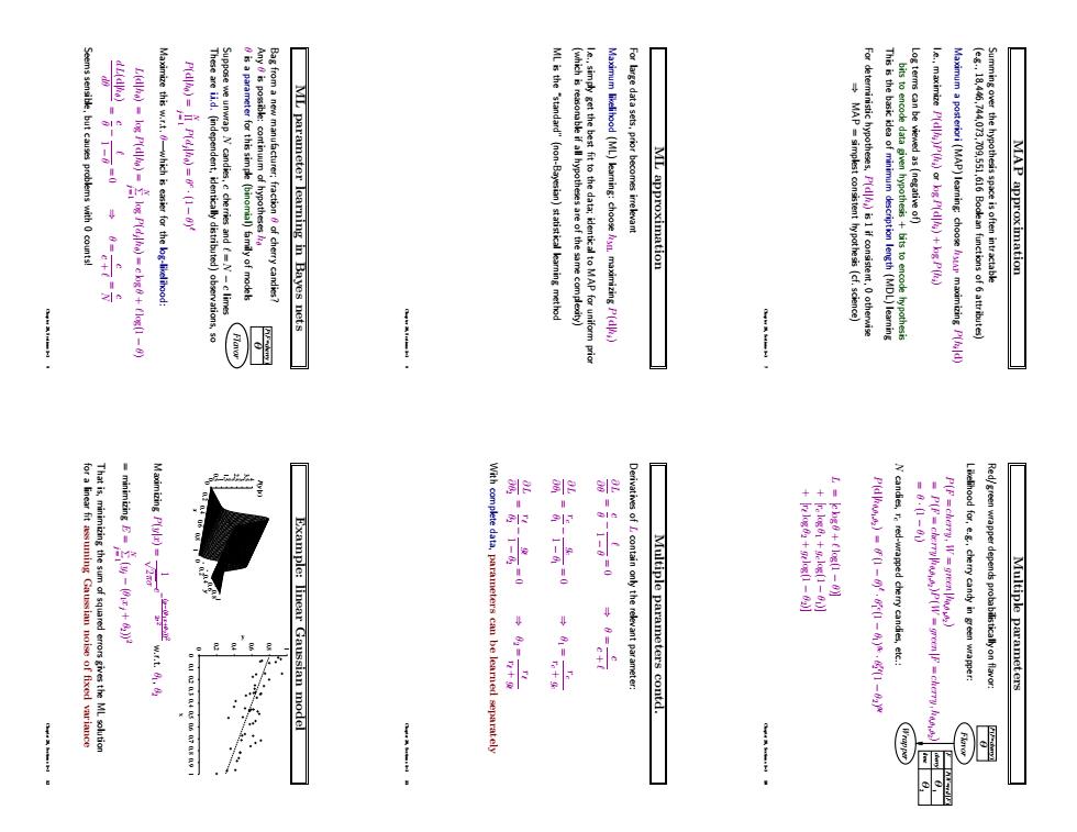
Seems sensible,but causes problems with 0 counts! . Maximize this w.r.t.0-which is easier for the lg-likelihood: These are ii.d.(independent,identically distributed)observations,so Suppose we unwrap N candies,c cherries and (=N-c limes is a parameter for this simple (binomial)family of model Any is possible:continuum of hypotheses Bag from a new manufacturer:fraction 8 of cherry candies? ML parameter learning in Bayes nets ML is the "standard"(non-Bayesian)statistical learning method (which is reasonable if all hypotheses are of the same complecity) le.,simply get the best fit to the data;identical to MAP for uniform prio Maximum likelihaod (ML)learning:choosen maximizing P(d) For large data sets,prior becomes irrelevant ML approximation MAP simplest consistent hypothesis (cf.science) For deterministic hypotheses,P(dis1 if consistent.otherwise This is the basic idea of minimum description length (MDL)learning bits to encode data giwen hypothesis bits to encode hypothesis Log terms can be viewed as (negative of) le.,maximize P(d(ar kg P(d)+kg P() Maximum a posteriori (MAP)learning:choose maimizing P(d) (e.g..18,446,744,073,709,551,616 Bodlean functions of 6 attributes) Summing over the hypothesis space is often intractable MAP approximation for a linear fit assuming Gaussian noise of fixed variance That is,minimizing the sum of squared errors gives the ML solution Derivatives of L contain only the relevant parameter: Multiple parameters contd. +F9+-E) N candies,r red-wrapped cherry candies,etc.: P(F =cherry,W=green llig) Likelihood for,e.g..cherry candy in green wrapper: Red/green wrapper depends probabilisticallyon flavor: w.r.t.8.8 Multiple parameters 1000400070802 Example:linear Gaussian model With complete data,parameters can be learned separatelyMAP approximation Summing over the hypothesis space is often intractable (e.g., 18,446,744,073,709,551,616 Boolean functions of 6 attributes) Maximum a posteriori (MAP) learning: choose hMAP maximizing P(hi |d) I.e., maximize P(d|hi)P(hi) or log P(d|hi) + log P(hi) Log terms can be viewed as (negative of) bits to encode data given hypothesis + bits to encode hypothesis This is the basic idea of minimum description length (MDL) learning For deterministic hypotheses, P(d|hi) is 1 if consistent, 0 otherwise ⇒ MAP = simplest consistent hypothesis (cf. science) Chapter 20, Sections 1–3 7 ML approximation For large data sets, prior becomes irrelevant Maximum likelihood (ML) learning: choose hML maximizing P(d|hi) I.e., simply get the best fit to the data; identical to MAP for uniform prior (which is reasonable if all hypotheses are of the same complexity) ML is the “standard” (non-Bayesian) statistical learning method Chapter 20, Sections 1–3 8 ML parameter learning in Bayes nets Bag from a new manufacturer; fraction θ of cherry candies? Flavor P F=cherry ( ) θ Any θ is possible: continuum of hypotheses hθ θ is a parameter for this simple (binomial) family of models Suppose we unwrap N candies, c cherries and ` = N − c limes These are i.i.d. (independent, identically distributed) observations, so P(d|hθ) = YN j = 1 P(dj |hθ) = θ c · (1 − θ) ` Maximize this w.r.t. θ—which is easier for the log-likelihood: L(d|hθ) = log P(d|hθ) = XN j = 1 log P(dj |hθ) = c log θ + ` log(1 − θ) dL(d|hθ) dθ = θ c − ` 1 − θ = 0 ⇒ θ = c c + ` = N c Seems sensible, but causes problems with 0 counts! Chapter 20, Sections 1–3 9 Multiple parameters Red/green wrapper depends probabilistically on flavor: P F=cherry ( ) Wrapper Flavor P( ) W=red | F cherry F 2 lime θ 1 θ θ Likelihood for, e.g., cherry candy in green wrapper: P(F = cherry, W = green|hθ,θ1,θ2 ) = P(F = cherry|hθ,θ1,θ2 )P(W = green|F = cherry, hθ,θ1,θ2 ) = θ · (1 − θ1) N candies, rc red-wrapped cherry candies, etc.: P(d|hθ,θ1,θ2 ) = θ c (1 − θ) ` · θ rc 1 (1 − θ1) gc · θ r` 2 (1 − θ2) g` L = [c log θ + ` log(1 − θ)] + [rc log θ1 + gc log(1 − θ1)] + [r` log θ2 + g` log(1 − θ2)] Chapter 20, Sections 1–3 10 Multiple parameters contd. Derivatives of L contain only the relevant parameter: ∂L ∂θ = θ c − ` 1 − θ = 0 ⇒ θ = c c + ` ∂L ∂θ1 = rc θ1 − gc 1 − θ1 = 0 ⇒ θ1 = rc rc + gc ∂L ∂θ2 = r` θ2 − g` 1 − θ2 = 0 ⇒ θ2 = r` r` + g` With complete data, parameters can be learned separately Chapter 20, Sections 1–3 11 Example: linear Gaussian model 0 0.2 0.4 0.6 0.8 1 x 0 0.2 0.4 0.6 0.8 1 y 0 0.5 1 1.5 2 2.5 3 3.5 4 P(y |x) 0 0.2 0.4 0.6 0.8 1 0 0.1 0.2 0.3 0.4 0.5 0.6 0.7 0.8 0.9 1 y x Maximizing P(y|x) = 1 √ 2πσ e − (y−(θ1 x+θ2 )) 2 2σ 2 w.r.t. θ1, θ2 = minimizing E = XN j = 1 (yj − (θ1xj + θ2)) 2 That is, minimizing the sum of squared errors gives the ML solution for a linear fit assuming Gaussian noise of fixed variance Chapter 20, Sections 1–3 12