正在加载图片...

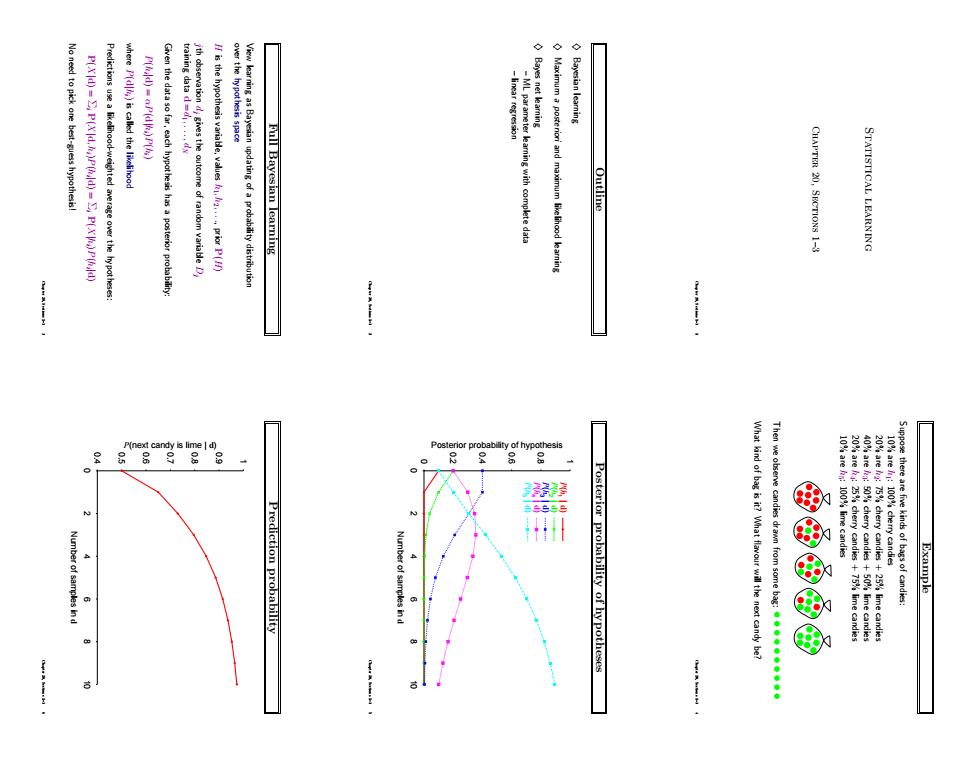
2 P(Xd)=E,P(Xld.P(d)=S,P(XP(d) P(d)is called the likelihe Full Bayesian learning STATISTICAL LEARNIN e observe candies dram from some bag:Statistical learning Chapter 20, Sections 1–3 Chapter 20, Sections 1–3 1 Outline ♦ Bayesian learning ♦ Maximum a posteriori and maximum likelihood learning ♦ Bayes net learning – ML parameter learning with complete data – linear regression Chapter 20, Sections 1–3 2 Full Bayesian learning View learning as Bayesian updating of a probability distribution over the hypothesis space H is the hypothesis variable, values h1, h2, . . ., prior P(H) jth observation dj gives the outcome of random variable Dj training data d = d1, . . . , dN Given the data so far, each hypothesis has a posterior probability: P(hi |d) = αP(d|hi)P(hi) where P(d|hi) is called the likelihood Predictions use a likelihood-weighted average over the hypotheses: P(X|d) = Σi P(X|d, hi)P(hi |d) = Σi P(X|hi)P(hi |d) No need to pick one best-guess hypothesis! Chapter 20, Sections 1–3 3 Example Suppose there are five kinds of bags of candies: 10% are h1: 100% cherry candies 20% are h2: 75% cherry candies + 25% lime candies 40% are h3: 50% cherry candies + 50% lime candies 20% are h4: 25% cherry candies + 75% lime candies 10% are h5: 100% lime candies Then we observe candies drawn from some bag: What kind of bag is it? What flavour will the next candy be? Chapter 20, Sections 1–3 4 Posterior probability of hypotheses 0 0.2 0.4 0.6 0.8 1 0 2 4 6 8 10 Posterior probability of hypothesis Number of samples in d P(h1 | d) P(h2 | d) P(h3 | d) P(h4 | d) P(h5 | d) Chapter 20, Sections 1–3 5 Prediction probability 0.4 0.5 0.6 0.7 0.8 0.9 1 0 2 4 6 8 10 P(next candy is lime | d) Number of samples in d Chapter 20, Sections 1–3 6