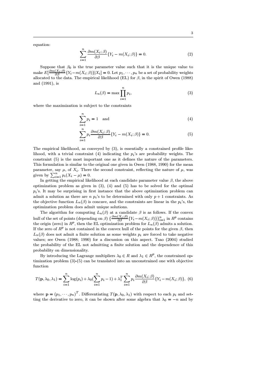
3 equation: Om(:(Y-m(X::))0. (2) 83 Suppose that Bo is the true parameter value such that it is the unique value to make Em(=0.Let p,n be a set of probability weights allocated to the data.The empirical likelihood(EL)for B,in the spirit of Owen(1988) and (1991),is Ln(a=maxΠpa, (3) =1 where the maximization is subject to the constraints ∑n=1aud (4) = .Om(XB)(Y:-m(X:B))=0. (5) 83 The empirical likelihood,as conveyed by (3),is essentially a constrained profile like- lihood,with a trivial constraint (4)indicating the p,'s are probability weights.The constraint (5)is the most important one as it defines the nature of the parameters This formulation is similar to the original one given in Owen(1988,1990)for the mean parameter,say u,of Xi.There the second constraint,reflecting the nature of u,was given by∑-1pi(X-)=0. In getting the empirical likelihood at each candidate parameter value B,the above optimization problem as given in (3),(4)and(5)has to be solved for the optimal Pi's.It may be surprising in first instance that the above optimization problem can admit a solution as there are n pi's to be determined with only p+1 constraints.As the objective function In(B)is concave,and the constraints are linear in the Pi's,the optimization problem does admit unique solutions. The algorithm for computing Ln(B)at a candidate B is as follows.If the convex hull of the set of points (depending on {mm(in RPcontains the origin(zero)in RP,then the EL optimization problem for Ln(B)admits a solution. If the zero of RP is not contained in the convex hull of the points for the given B,then Ln(B)does not admit a finite solution as some weights pi are forced to take negative values;see Owen (1988;1990)for a discussion on this aspect.Tsao (2004)studied the probability of the EL not admitting a finite solution and the dependence of this probability on dimensionality. By introducing the Lagrange multipliers Ao ER and AIE RP,the constrained op- timization problem (3)-(5)can be translated into an unconstrained one with objective function T(p,0,A1)=∑1og,)+o(∑P-1)+T∑p Om(XY:-m(XB)(6) 03 where p=(p1,n)T.Differentiating T(p,o,with respect to each pi and set- ting the derivative to zero,it can be shown after some algebra that Ao =-n and by3 equation: Xn i=1 ∂m(Xi ; β) ∂β {Yi − m(Xi ; β)} = 0. (2) Suppose that β0 is the true parameter value such that it is the unique value to make E[ ∂m(Xi;β) ∂β {Yi−m(Xi ; β)}|Xi ] = 0. Let p1, · · · , pn be a set of probability weights allocated to the data. The empirical likelihood (EL) for β, in the spirit of Owen (1988) and (1991), is Ln(β) = maxYn i=1 pi , (3) where the maximization is subject to the constraints Xn i=1 pi = 1 and (4) Xn i=1 pi ∂m(Xi ; β) ∂β {Yi − m(Xi ; β)} = 0. (5) The empirical likelihood, as conveyed by (3), is essentially a constrained profile like￾lihood, with a trivial constraint (4) indicating the pi ’s are probability weights. The constraint (5) is the most important one as it defines the nature of the parameters. This formulation is similar to the original one given in Owen (1988, 1990) for the mean parameter, say µ, of Xi . There the second constraint, reflecting the nature of µ, was given by Pn i=1 pi(Xi − µ) = 0. In getting the empirical likelihood at each candidate parameter value β, the above optimization problem as given in (3), (4) and (5) has to be solved for the optimal pi ’s. It may be surprising in first instance that the above optimization problem can admit a solution as there are n pi ’s to be determined with only p + 1 constraints. As the objective function Ln(β) is concave, and the constraints are linear in the pi ’s, the optimization problem does admit unique solutions. The algorithm for computing Ln(β) at a candidate β is as follows. If the convex hull of the set of points (depending on β) { ∂m(Xi;β) ∂β {Yi−m(Xi ; β)}}n i=1 in R p contains the origin (zero) in R p , then the EL optimization problem for Ln(β) admits a solution. If the zero of R p is not contained in the convex hull of the points for the given β, then Ln(β) does not admit a finite solution as some weights pi are forced to take negative values; see Owen (1988; 1990) for a discussion on this aspect. Tsao (2004) studied the probability of the EL not admitting a finite solution and the dependence of this probability on dimensionality. By introducing the Lagrange multipliers λ0 ∈ R and λ1 ∈ R p , the constrained op￾timization problem (3)-(5) can be translated into an unconstrained one with objective function T(p, λ0, λ1) = Xn i=1 log(pi) +λ0( Xn i=1 pi −1) +λ T 1 Xn i=1 pi ∂m(Xi ; β) ∂β {Yi − m(Xi ; β)}, (6) where p = (p1, · · · , pn) T . Differentiating T(p, λ0, λ1) with respect to each pi and set￾ting the derivative to zero, it can be shown after some algebra that λ0 = −n and by