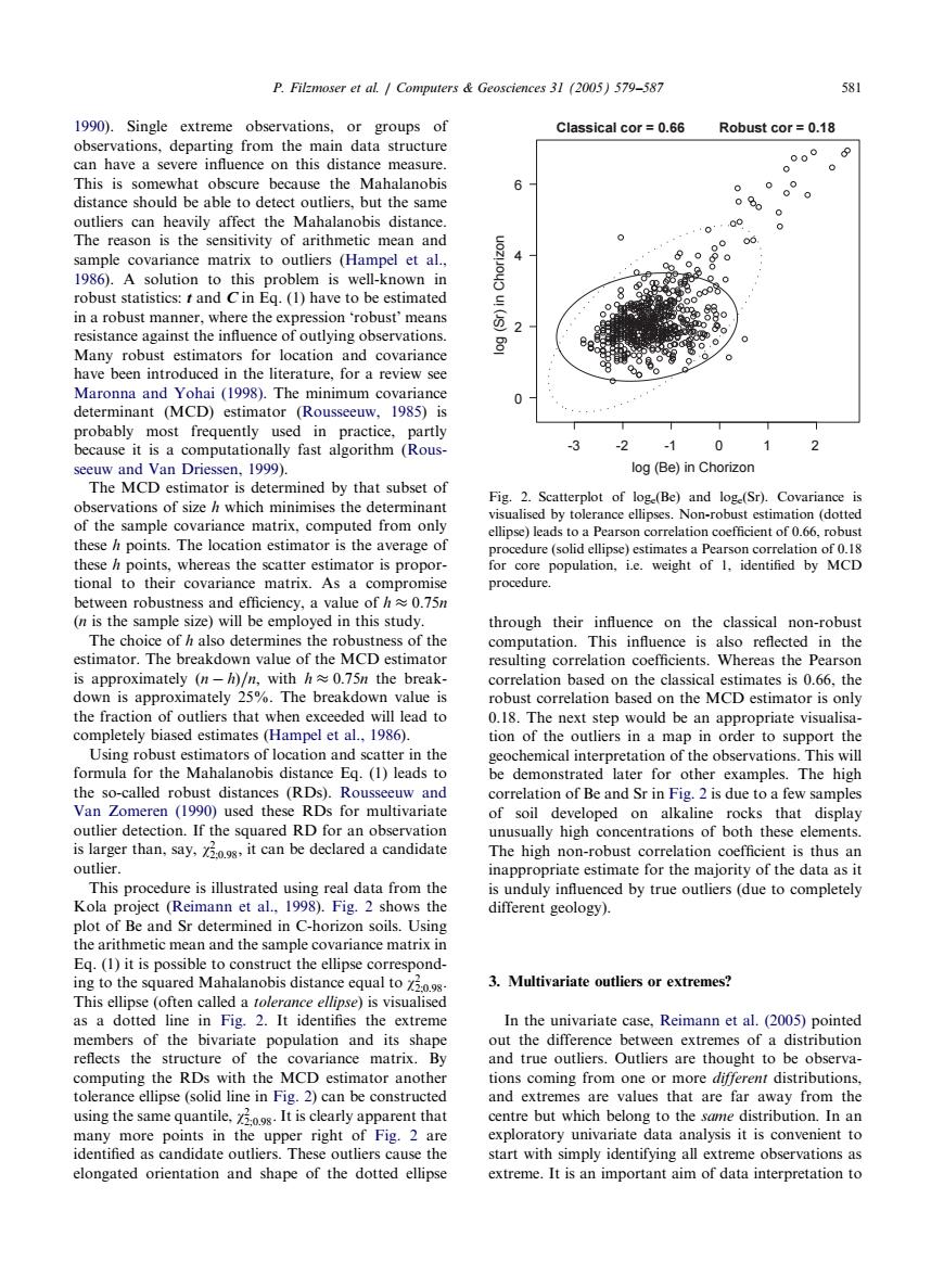
P.Filzmoser et al.Computers Geosciences 31 (2005)579-587 581 1990).Single extreme observations,or groups of Classical cor 0.66 Robust cor=0.18 observations,departing from the main data structure can have a severe influence on this distance measure. 000 This is somewhat obscure because the Mahalanobis distance should be able to detect outliers,but the same o60 0°。 outliers can heavily affect the Mahalanobis distance. 0 The reason is the sensitivity of arithmetic mean and 00 sample covariance matrix to outliers (Hampel et al., 4 1986).A solution to this problem is well-known in robust statistics:t and Cin Eq.(1)have to be estimated N in a robust manner.where the expression 'robust'means resistance against the influence of outlying observations. Many robust estimators for location and covariance have been introduced in the literature,for a review see Maronna and Yohai (1998).The minimum covariance determinant (MCD)estimator (Rousseeuw,1985)is probably most frequently used in practice,partly because it is a computationally fast algorithm (Rous- -3 -2 7 seeuw and Van Driessen,1999). log (Be)in Chorizon The MCD estimator is determined by that subset of Fig.2.Scatterplot of log (Be)and log (Sr).Covariance is observations of size h which minimises the determinant visualised by tolerance ellipses.Non-robust estimation (dotted of the sample covariance matrix,computed from only ellipse)leads to a Pearson correlation coefficient of 0.66,robust these h points.The location estimator is the average of procedure (solid ellipse)estimates a Pearson correlation of 0.18 these h points,whereas the scatter estimator is propor- for core population,i.e.weight of 1.identified by MCD tional to their covariance matrix.As a compromise procedure. between robustness and efficiency,a value of h0.75n (n is the sample size)will be employed in this study. through their influence on the classical non-robust The choice of h also determines the robustness of the computation.This influence is also reflected in the estimator.The breakdown value of the MCD estimator resulting correlation coefficients.Whereas the Pearson is approximately (n-h)/n,with h0.75n the break- correlation based on the classical estimates is 0.66.the down is approximately 25%.The breakdown value is robust correlation based on the MCD estimator is only the fraction of outliers that when exceeded will lead to 0.18.The next step would be an appropriate visualisa- completely biased estimates(Hampel et al.,1986). tion of the outliers in a map in order to support the Using robust estimators of location and scatter in the geochemical interpretation of the observations.This will formula for the Mahalanobis distance Eq.(1)leads to be demonstrated later for other examples.The high the so-called robust distances (RDs).Rousseeuw and correlation of Be and Sr in Fig.2 is due to a few samples Van Zomeren (1990)used these RDs for multivariate of soil developed on alkaline rocks that display outlier detection.If the squared RD for an observation unusually high concentrations of both these elements. is larger than,say,it can be declared a candidate The high non-robust correlation coefficient is thus an outlier. inappropriate estimate for the majority of the data as it This procedure is illustrated using real data from the is unduly influenced by true outliers (due to completely Kola project (Reimann et al.,1998).Fig.2 shows the different geology)】 plot of Be and Sr determined in C-horizon soils.Using the arithmetic mean and the sample covariance matrix in Eq.(1)it is possible to construct the ellipse correspond- ing to the squared Mahalanobis distance equal to 72.0.9s. 3.Multivariate outliers or extremes? This ellipse (often called a tolerance ellipse)is visualised as a dotted line in Fig.2.It identifies the extreme In the univariate case,Reimann et al.(2005)pointed members of the bivariate population and its shape out the difference between extremes of a distribution reflects the structure of the covariance matrix.By and true outliers.Outliers are thought to be observa- computing the RDs with the MCD estimator another tions coming from one or more different distributions, tolerance ellipse (solid line in Fig.2)can be constructed and extremes are values that are far away from the using the same quantile,29s.It is clearly apparent that centre but which belong to the same distribution.In an many more points in the upper right of Fig.2 are exploratory univariate data analysis it is convenient to identified as candidate outliers.These outliers cause the start with simply identifying all extreme observations as elongated orientation and shape of the dotted ellipse extreme.It is an important aim of data interpretation to1990). Single extreme observations, or groups of observations, departingfrom the main data structure can have a severe influence on this distance measure. This is somewhat obscure because the Mahalanobis distance should be able to detect outliers, but the same outliers can heavily affect the Mahalanobis distance. The reason is the sensitivity of arithmetic mean and sample covariance matrix to outliers (Hampel et al., 1986). A solution to this problem is well-known in robust statistics: t and C in Eq. (1) have to be estimated in a robust manner, where the expression ‘robust’ means resistance against the influence of outlying observations. Many robust estimators for location and covariance have been introduced in the literature, for a review see Maronna and Yohai (1998). The minimum covariance determinant (MCD) estimator (Rousseeuw, 1985) is probably most frequently used in practice, partly because it is a computationally fast algorithm (Rous￾seeuw and Van Driessen, 1999). The MCD estimator is determined by that subset of observations of size h which minimises the determinant of the sample covariance matrix, computed from only these h points. The location estimator is the average of these h points, whereas the scatter estimator is propor￾tional to their covariance matrix. As a compromise between robustness and efficiency, a value of h  0:75n (n is the sample size) will be employed in this study. The choice of h also determines the robustness of the estimator. The breakdown value of the MCD estimator is approximately ðn hÞ=n; with h  0:75n the break￾down is approximately 25%. The breakdown value is the fraction of outliers that when exceeded will lead to completely biased estimates (Hampel et al., 1986). Usingrobust estimators of location and scatter in the formula for the Mahalanobis distance Eq. (1) leads to the so-called robust distances (RDs). Rousseeuw and Van Zomeren (1990) used these RDs for multivariate outlier detection. If the squared RD for an observation is larger than, say, w2 2;0:98; it can be declared a candidate outlier. This procedure is illustrated usingreal data from the Kola project (Reimann et al., 1998). Fig. 2 shows the plot of Be and Sr determined in C-horizon soils. Using the arithmetic mean and the sample covariance matrix in Eq. (1) it is possible to construct the ellipse correspond￾ingto the squared Mahalanobis distance equal to w2 2;0:98: This ellipse (often called a tolerance ellipse) is visualised as a dotted line in Fig. 2. It identifies the extreme members of the bivariate population and its shape reflects the structure of the covariance matrix. By computingthe RDs with the MCD estimator another tolerance ellipse (solid line in Fig. 2) can be constructed usingthe same quantile, w2 2;0:98: It is clearly apparent that many more points in the upper right of Fig. 2 are identified as candidate outliers. These outliers cause the elongated orientation and shape of the dotted ellipse through their influence on the classical non-robust computation. This influence is also reflected in the resultingcorrelation coefficients. Whereas the Pearson correlation based on the classical estimates is 0.66, the robust correlation based on the MCD estimator is only 0.18. The next step would be an appropriate visualisa￾tion of the outliers in a map in order to support the geochemical interpretation of the observations. This will be demonstrated later for other examples. The high correlation of Be and Sr in Fig. 2 is due to a few samples of soil developed on alkaline rocks that display unusually high concentrations of both these elements. The high non-robust correlation coefficient is thus an inappropriate estimate for the majority of the data as it is unduly influenced by true outliers (due to completely different geology). 3. Multivariate outliers or extremes? In the univariate case, Reimann et al. (2005) pointed out the difference between extremes of a distribution and true outliers. Outliers are thought to be observa￾tions comingfrom one or more different distributions, and extremes are values that are far away from the centre but which belongto the same distribution. In an exploratory univariate data analysis it is convenient to start with simply identifyingall extreme observations as extreme. It is an important aim of data interpretation to ARTICLE IN PRESS -3 -2 -1 0 2 0 2 log (Be) in Chorizon log (Sr) in Chorizon Classical cor = 0.66 Robust cor = 0.18 4 6 1 Fig. 2. Scatterplot of loge(Be) and loge(Sr). Covariance is visualised by tolerance ellipses. Non-robust estimation (dotted ellipse) leads to a Pearson correlation coefficient of 0.66, robust procedure (solid ellipse) estimates a Pearson correlation of 0.18 for core population, i.e. weight of 1, identified by MCD procedure. P. Filzmoser et al. / Computers & Geosciences 31 (2005) 579–587 581