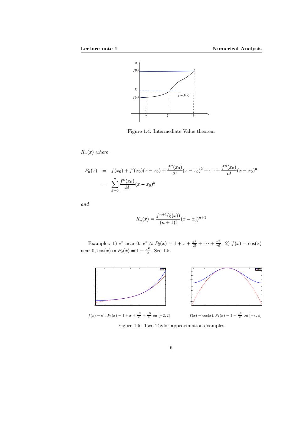
Lecture note 1 Numerical Analysis f6) f(a =f(r) Figure 1.4:Intermediate Value theorem Rn(r)where Pn(z)= fo+ole-0+"aolz-oP+…+严mle-or 2 n! ml红-o k=0 and R国=t1z-o+1 (n+1)！ Example::1)e near0:e2≈R(a)=1+x+分+…+元.2)fo)=cos( near0,cos()≈乃(d)=1-号，See1.5. fa)=e2,P乃(m)=1+x+号+om【-2,2习 f(a)=cos(e).PB(e)=1-号on【-T,可 Figure 1.5:Two Taylor approximation examplesLecture note 1 Numerical Analysis a ξ b y = f(x) x y f(b) f(a) K Figure 1.4: Intermediate Value theorem Rn(x) where Pn(x) = f(x0) + f ′ (x0)(x − x0) + f ′′(x0) 2! (x − x0) 2 + · · · + f n(x0) n! (x − x0) n = Xn k=0 f k (x0) k! (x − x0) k and Rn(x) = f n+1(ξ(x)) (n + 1)! (x − x0) n+1 Example:: 1) e x near 0: e x ≈ P3(x) = 1 + x + x 2 2! + · · · + x n n! . 2) f(x) = cos(x) near 0, cos(x) ≈ P2(x) = 1 − x 2 2 . See 1.5. −2 −1.5 −1 −0.5 0 0.5 1 1.5 2 −1 0 1 2 3 4 5 6 7 8 f(x)=exp(x) P3 (x) −3 −2 −1 0 1 2 3 −4 −3.5 −3 −2.5 −2 −1.5 −1 −0.5 0 0.5 1 f(x)=cos(x) P2 (x)=1−1/2 x2 f(x) = e x , P3(x) = 1 + x + x 2 2! + x 3 3! on [−2, 2] f(x) = cos(x), P2(x) = 1 − x 2 2 on [−π, π] Figure 1.5: Two Taylor approximation examples 6