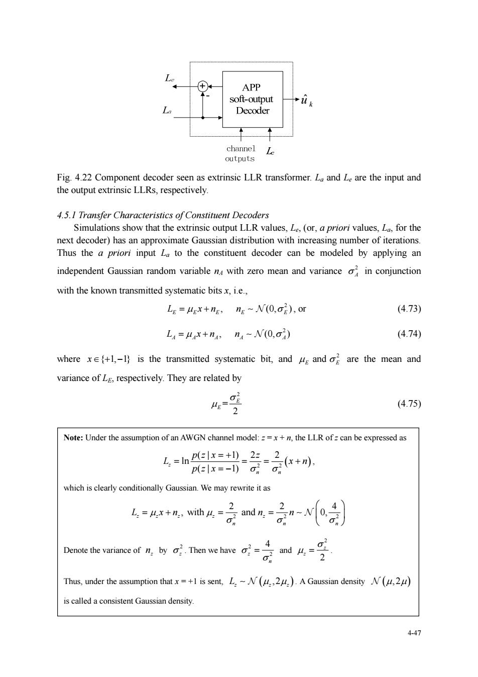
APP soft-output Decoder channel Le Fig.4.22 Component decoder seen as extrinsic LLR transformer.L and L are the input and the output extrinsic LLRs,respectively. 4.5.I Transfer Characteristics ofConstituent Decoders Simulations show that the extrinsic output LLR values,L(values,for the next decoder)has an approximate Gaussian distribution with increasing number of iterations. Thus the a priori input La to the constituent decoder can be modeled by applying an independent Gaussian random variable n with zero mean and variance in conjunction with the known transmitted systematic bitsx,i.e Lg=ugx+ng,ng-N(0.ag),or (4.73) L=x+n n-N(0i) (4.74) where xe+-1)is the transmitted systematic bit,and and are the mean and variance ofLrespectively.They are related by (4.75) Note:Under the assumption of an AWGN channel model:x+nthe LLR of=can be expressed as L=helx=+_2三。2 =lx=-(). which isclearly conditionally Gaussian.We may rewrite it as L.=ux+n,with u, 2 2 ef风e ac hae矿-是化-号 Thus.under the assumption thatx=+1 is sent.L.~(u).A Gaussian density (u2u) iscalled a consistent Gaussian density. 447 4-47 u k ˆ Fig. 4.22 Component decoder seen as extrinsic LLR transformer. La and Le are the input and the output extrinsic LLRs, respectively. 4.5.1 Transfer Characteristics of Constituent Decoders Simulations show that the extrinsic output LLR values, Le, (or, a priori values, La, for the next decoder) has an approximate Gaussian distribution with increasing number of iterations. Thus the a priori input La to the constituent decoder can be modeled by applying an independent Gaussian random variable nA with zero mean and variance 2  A in conjunction with the known transmitted systematic bits x, i.e., 2 , (0, ) L xn n EE E E E       , or (4.73) 2 , (0, ) L xn n AA A A A       (4.74) where { 1, 1} x  is the transmitted systematic bit, and 2 and  E E  are the mean and variance of LE, respectively. They are related by 2 = 2 E E   (4.75) Note: Under the assumption of an AWGN channel model: z = x + n, the LLR of z can be expressed as   2 2 ( | 1) 2 2 ln ( | 1) z n n pz x z L xn pz x          , which is clearly conditionally Gaussian. We may rewrite it as 22 2 22 4 , with and 0, zz z z z nn n L xn n n                 Denote the variance of z n by 2  z . Then we have 2 2 4 z n    and 2 2 z z    . Thus, under the assumption that x = +1 is sent,  ,2  Lz zz     . A Gaussian density    ,2 is called a consistent Gaussian density