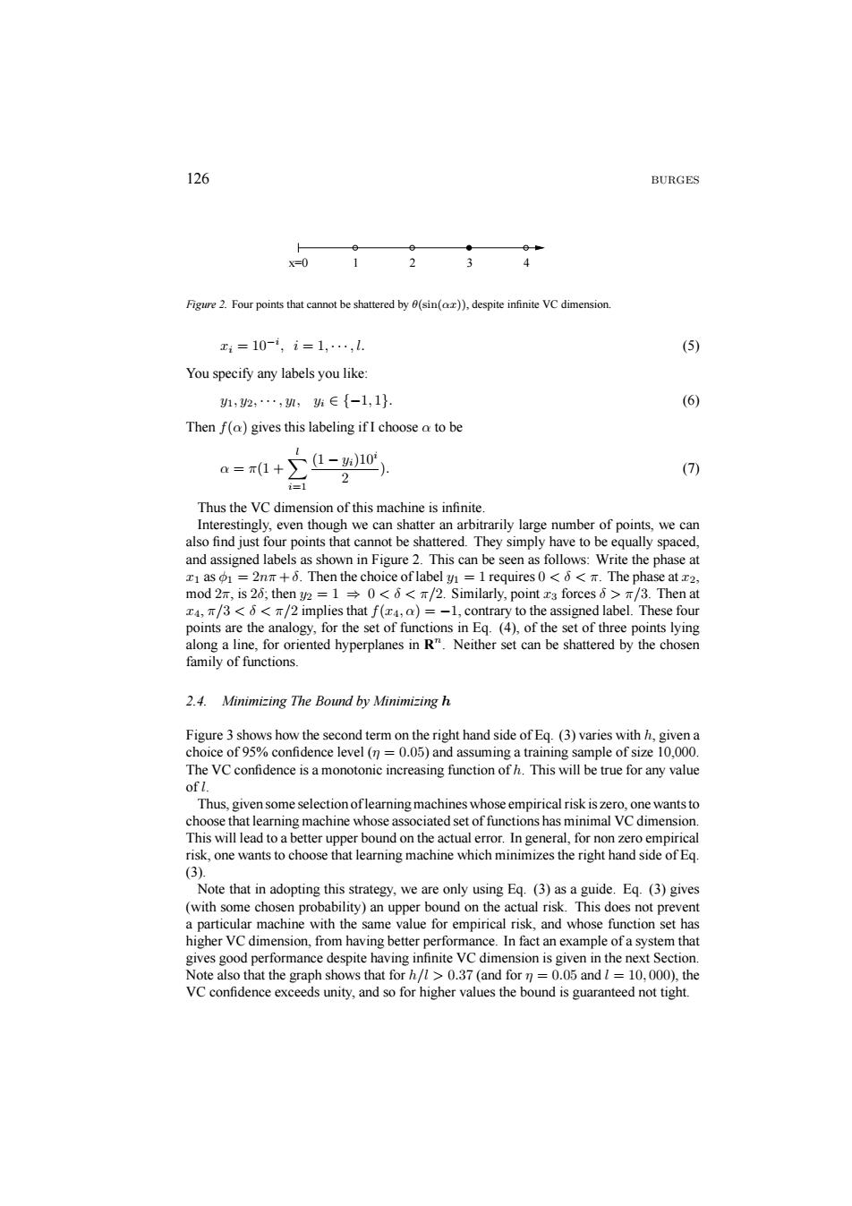
126 BURGES 人 x=0 1 2 Figure 2.Four points that cannot be shattered by 0(sin()),despite infinite VC dimension x1=10-i,i=1,…,l. (5) You specify any labels you like 1,2,…,,∈{-1,1} (6) Then f(a)gives this labeling if I choose a to be a=π1+∑-h10 (7) 2 Thus the VC dimension of this machine is infinite. Interestingly,even though we can shatter an arbitrarily large number of points,we can also find just four points that cannot be shattered.They simply have to be equally spaced, and assigned labels as shown in Figure 2.This can be seen as follows:Write the phase at xI as o1=2nm+0.Then the choice of label y =1 requires 0<o<T.The phase at x2. mod 2n,is 26;then y2 =10<6</2.Similarly,point z3 forces 6>/3.Then at x4,/3<6<T/2 implies that f(x4,a)=-1,contrary to the assigned label.These four points are the analogy,for the set of functions in Eq.(4),of the set of three points lying along a line,for oriented hyperplanes in R".Neither set can be shattered by the chosen family of functions. 2.4.Minimizing The Bound by Minimizing h Figure 3 shows how the second term on the right hand side of Eq.(3)varies with h,given a choice of 95%confidence level (n=0.05)and assuming a training sample of size 10,000. The VC confidence is a monotonic increasing function of h.This will be true for any value of l. Thus,given some selection oflearning machines whose empirical risk is zero,one wants to choose that learning machine whose associated set of functions has minimal VC dimension. This will lead to a better upper bound on the actual error.In general,for non zero empirical risk,one wants to choose that learning machine which minimizes the right hand side of Eq. (3) Note that in adopting this strategy,we are only using Eq.(3)as a guide.Eq.(3)gives (with some chosen probability)an upper bound on the actual risk.This does not prevent a particular machine with the same value for empirical risk,and whose function set has higher VC dimension,from having better performance.In fact an example of a system that gives good performance despite having infinite VC dimension is given in the next Section. Note also that the graph shows that for h/>0.37 (and for n =0.05 and l 10,000),the VC confidence exceeds unity,and so for higher values the bound is guaranteed not tight.126 BURGES x=0 1234 Figure 2. Four points that cannot be shattered by θ(sin(αx)), despite infinite VC dimension. xi = 10−i , i = 1, ··· ,l. (5) You specify any labels you like: y1, y2, ··· , yl, yi ∈ {−1, 1}. (6) Then f(α) gives this labeling if I choose α to be α = π(1 +X l i=1 (1 − yi)10i 2 ). (7) Thus the VC dimension of this machine is infinite. Interestingly, even though we can shatter an arbitrarily large number of points, we can also find just four points that cannot be shattered. They simply have to be equally spaced, and assigned labels as shown in Figure 2. This can be seen as follows: Write the phase at x1 as φ1 = 2nπ +δ. Then the choice of label y1 = 1 requires 0 <δ<π. The phase at x2, mod 2π, is 2δ; then y2 = 1 ⇒ 0 < δ < π/2. Similarly, point x3 forces δ > π/3. Then at x4, π/3 < δ < π/2 implies that f(x4, α) = −1, contrary to the assigned label. These four points are the analogy, for the set of functions in Eq. (4), of the set of three points lying along a line, for oriented hyperplanes in Rn. Neither set can be shattered by the chosen family of functions. 2.4. Minimizing The Bound by Minimizing h Figure 3 shows how the second term on the right hand side of Eq. (3) varies with h, given a choice of 95% confidence level (η = 0.05) and assuming a training sample of size 10,000. The VC confidence is a monotonic increasing function of h. This will be true for any value of l. Thus, given some selection of learning machines whose empirical risk is zero, one wants to choose that learning machine whose associated set of functions has minimal VC dimension. This will lead to a better upper bound on the actual error. In general, for non zero empirical risk, one wants to choose that learning machine which minimizes the right hand side of Eq. (3). Note that in adopting this strategy, we are only using Eq. (3) as a guide. Eq. (3) gives (with some chosen probability) an upper bound on the actual risk. This does not prevent a particular machine with the same value for empirical risk, and whose function set has higher VC dimension, from having better performance. In fact an example of a system that gives good performance despite having infinite VC dimension is given in the next Section. Note also that the graph shows that for h/l > 0.37 (and for η = 0.05 and l = 10, 000), the VC confidence exceeds unity, and so for higher values the bound is guaranteed not tight