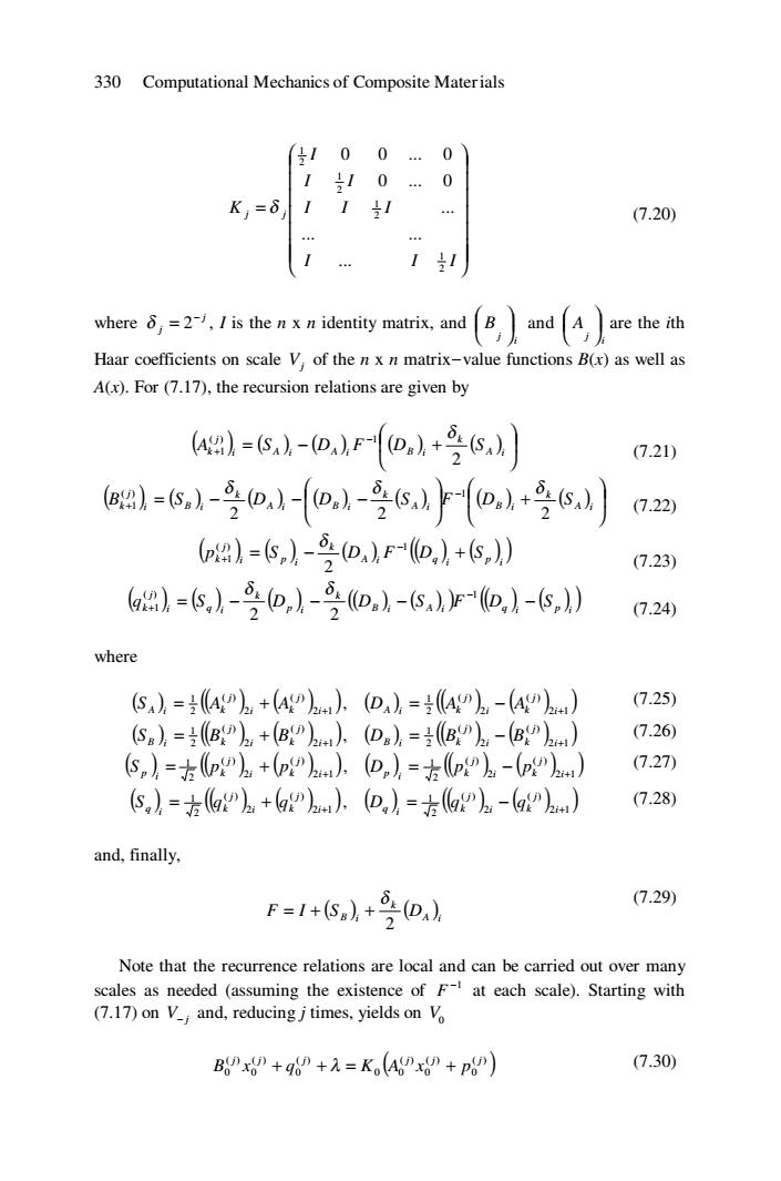
330 Computational Mechanics of Composite Materials 0 0 0 1 0 0 K,=δ 1 (7.20) 4 1 where is the identity matrix.andB and are the h Haar coefficients on scale V;of the n x n matrix-value functions B(x)as well as A(x).For(7.17),the recursion relations are given by =6,-D,r-o,+9, (7.21) ()--0--6))6 (7.22) =6)-DFD,)+6,》 (7.23) %,=6,-o,)-(D,-6F-o,-s,》 (7.24) where Sa,=49+a9),(D,=4b-(49h) (7.25) SB,=(B”+(BPh)(Ds),=BPA-(Bb） (7.26) sn)=古ph+(ph,(D,=方ph-(p） (7.27) (S,】=方aPa+gP）.(D,)=方aPh-gPh） (7.28) and,finally, F=1+5+受D (7.29) Note that the recurrence relations are local and can be carried out over many scales as needed (assuming the existence of F at each scale).Starting with (7.17)on V and,reducing jtimes.yields on V Bx8”+q8+=KAx+p） (7.30)330 Computational Mechanics of Composite Materials ⎟ ⎟ ⎟ ⎟ ⎟ ⎟ ⎟ ⎠ ⎞ ⎜ ⎜ ⎜ ⎜ ⎜ ⎜ ⎜ ⎝ ⎛ = I I I I I I I I I K j j 2 1 2 1 2 1 2 1 ... ... ... ... 0 ... 0 0 0 ... 0 δ (7.20) where j j − δ = 2 , I is the n x n identity matrix, and i j B ⎟ ⎠ ⎞ ⎜ ⎝ ⎛ and i j A ⎟ ⎠ ⎞ ⎜ ⎝ ⎛ are the ith Haar coefficients on scale Vj of the n x n matrix-value functions B(x) as well as A(x). For (7.17), the recursion relations are given by ( ) ()( ) ( ) ( ) ⎟ ⎠ ⎞ ⎜ ⎝ ⎛ = − + − + A i k i A i A i B i j Ak S D F D S 2 ( ) 1 1 δ (7.21) ( ) ( ) () () () ( ) ( ) ⎟ ⎠ ⎞ ⎜ ⎝ ⎛ ⎟ + ⎠ ⎞ ⎜ ⎝ ⎛ = − − − − + A i k A i B i k A i B i k i B i j Bk S D D S F D S 2 2 2 ( ) 1 1 δ δ δ (7.22) ( ) ( ) ( ) ( ) () ()i p i A i q k i i p j k p = S − D F D + S − + ( ) 1 1 2 δ (7.23) ( ) ( ) ( ) ( ) ( )() ( ) ()()i p i B i A i q k i p k i i q j k q = S − D − D − S F D − S − + ( ) 1 1 2 2 δ δ (7.24) where ( ) ( ) ()()2 1 ( ) 2 ( ) 2 1 + = + i j i k j S A i Ak A , ( ) ( ) ()()2 1 ( ) 2 ( ) 2 1 + = − i j i k j DA i Ak A (7.25) ( ) ( ) ()()2 1 ( ) 2 ( ) 2 1 + = + i j i k j S B i Bk B , ( ) ( ) ()()2 1 ( ) 2 ( ) 2 1 + = − i j i k j DB i Bk B (7.26) ( ) ( ) ()()2 1 ( ) 2 ( ) 2 1 + = + i j i k j k i S p p p , ( ) ( ) ()()2 1 ( ) 2 ( ) 2 1 + = − i j i k j k i Dp p p (7.27) ( ) ( ) ()()2 1 ( ) 2 ( ) 2 1 + = + i j i k j k i Sq q q , ( ) ( ) ()()2 1 ( ) 2 ( ) 2 1 + = − i j i k j k i Dq q q (7.28) and, finally, ( ) ( ) A i k F I S B i D 2 δ = + + (7.29) Note that the recurrence relations are local and can be carried out over many scales as needed (assuming the existence of −1 F at each scale). Starting with (7.17) on V− j and, reducing j times, yields on V0 ( ) ( ) 0 ( ) 0 ( ) 0 0 ( ) 0 ( ) 0 ( ) 0 j j j j j j B x + q + λ = K A x + p (7.30)