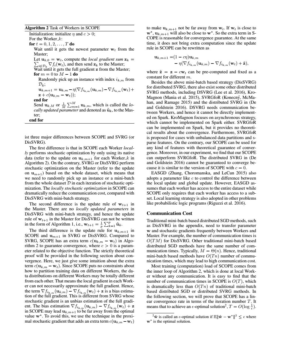
Algorithm 2 Task of Workers in SCOPE to make uk.m+1 not be far away from wt.If w:is close to Initialization:initialize n and c >0; w*.uk.m+1 will also be close to w*.So the extra term in S- For the Worker_: COPE is reasonable for convergence guarantee.At the same fort =0,1,2,...,T do time,it does not bring extra computation since the update Wait until it gets the newest parameter w:from the rule in SCOPE can be rewritten as Master; Let uk.o wt,compute the local gradient sum zk uk.m+1 =(1-cn)uk.m CiD Vfi(w:),and then send zk to the Master; -n(V fik.m (uk,m)-V fik.m (wt)+2), Wait until it gets the full gradient z from the Master: for m=0to M-1 do where 2=z-cwt can be pre-computed and fixed as a constant for different m. Randomly pick up an instance with index ik,m from Dk: Besides the above mini-batch based strategy (DisSVRG) uk.m+1=uk.m-n(V fis.m (uk,m)-V fix.m (wt)+ for distributed SVRG,there also exist some other distributed z+c(uk,m-wi)); SVRG methods,including DSVRG (Lee et al.2016).Kro- end for Magnon (Mania et al.2015),SVRGfoR (Konecny,McMa- Sendu.or which is called the lo han,and Ramage 2015)and the distributed SVRG in (De and Goldstein 2016).DSVRG needs communication be- cally updated parameter and denoted as uk,to the Mas- tween Workers,and hence it cannot be directly implement- ter; ed on Spark.KroMagnon focuses on asynchronous strategy, end for which cannot be implemented on Spark either.SVRGfoR can be implemented on Spark,but it provides no theoreti- cal results about the convergence.Furthermore,SVRGfoR ist three major differences between SCOPE and SVRG(or is proposed for cases with unbalanced data partitions and s- DisSVRG). parse features.On the contrary,our SCOPE can be used for The first difference is that in SCOPE each Worker local- any kind of features with theoretical guarantee of conver- ly performs stochastic optimization by only using its native gence.Moreover,in our experiment,we find that our SCOPE data (refer to the update on uk.m+1 for each Worker k in can outperform SVRGfoR.The distributed SVRG in (De Algorithm 2).On the contrary,SVRG or DisSVRG perform and Goldstein 2016)cannot be guaranteed to converge be- stochastic optimization on the Master (refer to the update cause it is similar to the version of SCOPE with c=0. on um+1)based on the whole dataset,which means that EASGD (Zhang,Choromanska,and LeCun 2015)also we need to randomly pick up an instance or a mini-batch adopts a parameter like c to control the difference between from the whole dataset D in each iteration of stochastic opti- the local update and global update.However,EASGD as- mization.The locally stochastic optimization in SCOPE can sumes that each worker has access to the entire dataset while dramatically reduce the communication cost,compared with SCOPE only requires that each worker has access to a sub- DisS VRG with mini-batch strategy. set.Local learning strategy is also adopted in other problems The second difference is the update rule of wt+1 in like probabilistic logic programs(Riguzzi et al.2016) the Master.There are no locally updated parameters in DisSVRG with mini-batch strategy,and hence the update Communication Cost rule of wi+1 in the Master for DisSVRG can not be written Traditional mini-batch based distributed SGD methods.such in the form of Algorithm,1i.e,wt+1=是∑k=1ik. as DisSVRG in the appendix,need to transfer parameter The third difference is the update rule for uk.m+1 in w and stochastic gradients frequently between Workers and SCOPE and um+1 in SVRG or DisSVRG.Compared to Master.For example,the number of communication times is SVRG,SCOPE has an extra term c(uk.m-wt)in Algo- O(TM)for DisSVRG.Other traditional mini-batch based rithm 2 to guarantee convergence,where c >0 is a param- distributed SGD methods have the same number of com- eter related to the objective function.The strictly theoretical munication times.Typically,M=e(n).Hence,traditional proof will be provided in the following section about con- mini-batch based methods have O(Tn)number of commu- vergence.Here,we just give some intuition about the extra nication times,which may lead to high communication cost term c(uk.m-wi).Since SCOPE puts no constraints about Most training(computation)load of SCOPE comes from how to partition training data on different Workers,the da- the inner loop of Algorithm 2,which is done at local Work- ta distributions on different Workers may be totally different er without any communication.It is easy to find that the from each other.That means the local gradient in each Work- number of communication times in SCOPE is O(T),which er can not necessarily approximate the full gradient.Hence, is dramatically less than O(Tn)of traditional mini-batch the term Vfi.(uk.m)-Vfis.(wt)+z is a bias estima- based distributed SGD or distributed SVRG methods.In tion of the full gradient.This is different from SVRG whose the following section,we will prove that SCOPE has a lin- stochastic gradient is an unbias estimation of the full gradi- ent.The bias estimation Vf(uk.m)-Vf(wt)+ ear convergence rate in terms of the iteration number T.It means that to achieve an e-optimal solution2,T=O(log). in SCOPE may lead uk.m+1 to be far away from the optimal value w*.To avoid this,we use the technique in the proxi- 2w is called an e-optimal solution ifEllw-w*l2 e where mal stochastic gradient that adds an extra term c(uk.m-wt) w*is the optimal solution.Algorithm 2 Task of Workers in SCOPE Initialization: initialize η and c > 0; For the Worker k: for t = 0, 1, 2, . . . , T do Wait until it gets the newest parameter wt from the Master; Let P uk,0 = wt, compute the local gradient sum zk = i∈Dk ∇fi(wt), and then send zk to the Master; Wait until it gets the full gradient z from the Master; for m = 0 to M − 1 do Randomly pick up an instance with index ik,m from Dk; uk,m+1 = uk,m −η(∇fik,m(uk,m)−∇fik,m(wt)+ z + c(uk,m − wt)); end for Send uk,M or 1 M PM m=1 uk,m, which is called the lo￾cally updated parameter and denoted as u˜k, to the Mas￾ter; end for ist three major differences between SCOPE and SVRG (or DisSVRG). The first difference is that in SCOPE each Worker local￾ly performs stochastic optimization by only using its native data (refer to the update on uk,m+1 for each Worker k in Algorithm 2). On the contrary, SVRG or DisSVRG perform stochastic optimization on the Master (refer to the update on um+1) based on the whole dataset, which means that we need to randomly pick up an instance or a mini-batch from the whole dataset D in each iteration of stochastic opti￾mization. The locally stochastic optimization in SCOPE can dramatically reduce the communication cost, compared with DisSVRG with mini-batch strategy. The second difference is the update rule of wt+1 in the Master. There are no locally updated parameters in DisSVRG with mini-batch strategy, and hence the update rule of wt+1 in the Master for DisSVRG can not be written in the form of Algorithm 1, i.e., wt+1 = 1 p Pp k=1 u˜k. The third difference is the update rule for uk,m+1 in SCOPE and um+1 in SVRG or DisSVRG. Compared to SVRG, SCOPE has an extra term c(uk,m − wt) in Algo￾rithm 2 to guarantee convergence, where c > 0 is a param￾eter related to the objective function. The strictly theoretical proof will be provided in the following section about con￾vergence. Here, we just give some intuition about the extra term c(uk,m − wt). Since SCOPE puts no constraints about how to partition training data on different Workers, the da￾ta distributions on different Workers may be totally different from each other. That means the local gradient in each Work￾er can not necessarily approximate the full gradient. Hence, the term ∇fik,m(uk,m) − ∇fik,m(wt) + z is a bias estima￾tion of the full gradient. This is different from SVRG whose stochastic gradient is an unbias estimation of the full gradi￾ent. The bias estimation ∇fik,m(uk,m) − ∇fik,m(wt) + z in SCOPE may lead uk,m+1 to be far away from the optimal value w∗ . To avoid this, we use the technique in the proxi￾mal stochastic gradient that adds an extra term c(uk,m −wt) to make uk,m+1 not be far away from wt. If wt is close to w∗ , uk,m+1 will also be close to w∗ . So the extra term in S￾COPE is reasonable for convergence guarantee. At the same time, it does not bring extra computation since the update rule in SCOPE can be rewritten as uk,m+1 =(1 − cη)uk,m − η(∇fik,m(uk,m) − ∇fik,m(wt) + zˆ), where zˆ = z − cwt can be pre-computed and fixed as a constant for different m. Besides the above mini-batch based strategy (DisSVRG) for distributed SVRG, there also exist some other distributed SVRG methods, including DSVRG (Lee et al. 2016), Kro￾Magnon (Mania et al. 2015), SVRGfoR (Konecny, McMa- ´ han, and Ramage 2015) and the distributed SVRG in (De and Goldstein 2016). DSVRG needs communication be￾tween Workers, and hence it cannot be directly implement￾ed on Spark. KroMagnon focuses on asynchronous strategy, which cannot be implemented on Spark either. SVRGfoR can be implemented on Spark, but it provides no theoreti￾cal results about the convergence. Furthermore, SVRGfoR is proposed for cases with unbalanced data partitions and s￾parse features. On the contrary, our SCOPE can be used for any kind of features with theoretical guarantee of conver￾gence. Moreover, in our experiment, we find that our SCOPE can outperform SVRGfoR. The distributed SVRG in (De and Goldstein 2016) cannot be guaranteed to converge be￾cause it is similar to the version of SCOPE with c = 0. EASGD (Zhang, Choromanska, and LeCun 2015) also adopts a parameter like c to control the difference between the local update and global update. However, EASGD as￾sumes that each worker has access to the entire dataset while SCOPE only requires that each worker has access to a sub￾set. Local learning strategy is also adopted in other problems like probabilistic logic programs (Riguzzi et al. 2016). Communication Cost Traditional mini-batch based distributed SGD methods, such as DisSVRG in the appendix, need to transfer parameter w and stochastic gradients frequently between Workers and Master. For example, the number of communication times is O(TM) for DisSVRG. Other traditional mini-batch based distributed SGD methods have the same number of com￾munication times. Typically, M = Θ(n). Hence, traditional mini-batch based methods have O(T n) number of commu￾nication times, which may lead to high communication cost. Most training (computation) load of SCOPE comes from the inner loop of Algorithm 2, which is done at local Work￾er without any communication. It is easy to find that the number of communication times in SCOPE is O(T), which is dramatically less than O(T n) of traditional mini-batch based distributed SGD or distributed SVRG methods. In the following section, we will prove that SCOPE has a lin￾ear convergence rate in terms of the iteration number T. It means that to achieve an -optimal solution2 , T = O(log 1  ). 2wˆ is called an -optimal solution if Ekwˆ − w∗ k 2 ≤  where w∗ is the optimal solution