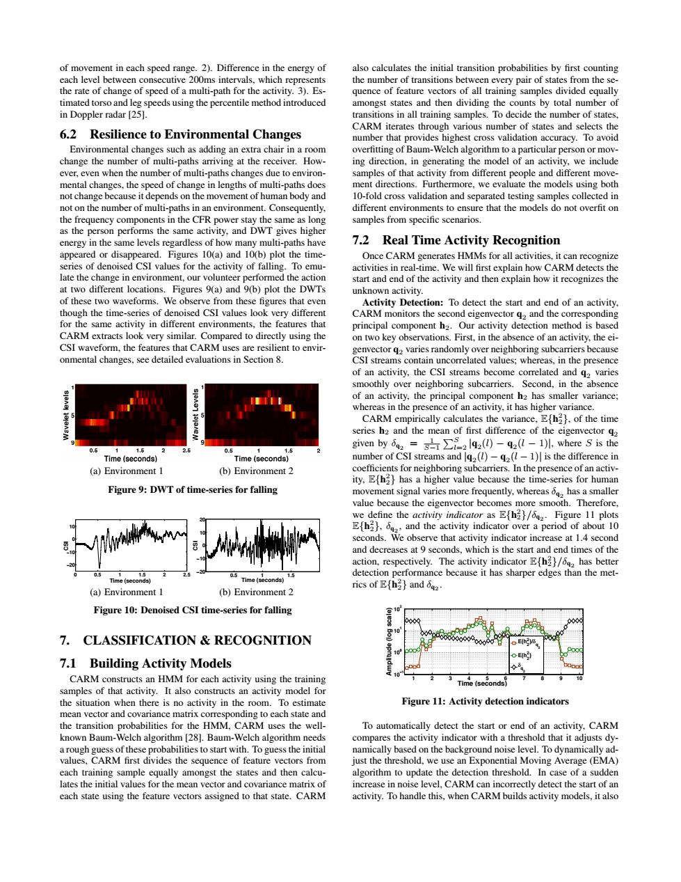
of movement in each speed range.2).Difference in the energy of also calculates the initial transition probabilities by first counting each level between consecutive 200ms intervals,which represents the number of transitions between every pair of states from the se- the rate of change of speed of a multi-path for the activity.3).Es- quence of feature vectors of all training samples divided equally timated torso and leg speeds using the percentile method introduced amongst states and then dividing the counts by total number of in Doppler radar [25]. transitions in all training samples.To decide the number of states. CARM iterates through various number of states and selects the 6.2 Resilience to Environmental Changes number that provides highest cross validation accuracy.To avoid Environmental changes such as adding an extra chair in a room overfitting of Baum-Welch algorithm to a particular person or mov- change the number of multi-paths arriving at the receiver.How- ing direction,in generating the model of an activity,we include ever,even when the number of multi-paths changes due to environ- samples of that activity from different people and different move- mental changes,the speed of change in lengths of multi-paths does ment directions.Furthermore,we evaluate the models using both not change because it depends on the movement of human body and 10-fold cross validation and separated testing samples collected in not on the number of multi-paths in an environment.Consequently, different environments to ensure that the models do not overfit on the frequency components in the CFR power stay the same as long samples from specific scenarios. as the person performs the same activity,and DWT gives higher energy in the same levels regardless of how many multi-paths have 7.2 Real Time Activity Recognition appeared or disappeared.Figures 10(a)and 10(b)plot the time- Once CARM generates HMMs for all activities,it can recognize series of denoised CSI values for the activity of falling.To emu activities in real-time.We will first explain how CARM detects the late the change in environment,our volunteer performed the action start and end of the activity and then explain how it recognizes the at two different locations.Figures 9(a)and 9(b)plot the DWTs unknown activity. of these two waveforms.We observe from these figures that even Activity Detection:To detect the start and end of an activity. though the time-series of denoised CSI values look very different CARM monitors the second eigenvector q2 and the corresponding for the same activity in different environments,the features that principal component h2.Our activity detection method is based CARM extracts look very similar.Compared to directly using the on two key observations.First,in the absence of an activity,the ei- CSI waveform.the features that CARM uses are resilient to envir- genvector q2 varies randomly over neighboring subcarriers because onmental changes,see detailed evaluations in Section 8. CSI streams contain uncorrelated values;whereas,in the presence of an activity,the CSI streams become correlated and q2 varies smoothly over neighboring subcarriers.Second,in the absence of an activity,the principal component h2 has smaller variance; whereas in the presence of an activity,it has higher variance. CARM empirically calculates the variance,Eh2).of the time series h2 and the mean of first difference of the eigenvector q2 06 1.6 05 1.5 given by2=s六∑L2l4z()-4el-1 where S is the Time (seconds) Time (seconds) number of CSI streams and q2(l)-q2(I-1)I is the difference in (a)Environment 1 (b)Environment 2 coefficients for neighboring subcarriers.In the presence of an activ- ity,Efh2 has a higher value because the time-series for human Figure 9:DWT of time-series for falling movement signal varies more frequently,whereas has a smaller value because the eigenvector becomes more smooth.Therefore. we define the activity indicator as E(h)/62.Figure 11 plots E(h.and the activity indicator over a period of about 10 seconds.We observe that activity indicator increase at 1.4 second and decreases at 9 seconds,which is the start and end times of the action,respectively.The activity indicator Efh2/has better 15 detection performance because it has sharper edges than the met- Time(seconds) Time(conds rics of E(h2}and 62 (a)Environment 1 (b)Environment 2 Figure 10:Denoised CSI time-series for falling 7.CLASSIFICATION RECOGNITION E(hM oh的 7.1 Building Activity Models CARM constructs an HMM for each activity using the training Time (seconds) samples of that activity.It also constructs an activity model for the situation when there is no activity in the room.To estimate Figure 11:Activity detection indicators mean vector and covariance matrix corresponding to each state and the transition probabilities for the HMM,CARM uses the well- To automatically detect the start or end of an activity.CARM known Baum-Welch algorithm[28].Baum-Welch algorithm needs compares the activity indicator with a threshold that it adjusts dy. a rough guess of these probabilities to start with.To guess the initial namically based on the background noise level.To dynamically ad- values,CARM first divides the sequence of feature vectors from just the threshold,we use an Exponential Moving Average (EMA) each training sample equally amongst the states and then calcu- algorithm to update the detection threshold.In case of a sudden lates the initial values for the mean vector and covariance matrix of increase in noise level,CARM can incorrectly detect the start of an each state using the feature vectors assigned to that state.CARM activity.To handle this,when CARM builds activity models,it alsoof movement in each speed range. 2). Difference in the energy of each level between consecutive 200ms intervals, which represents the rate of change of speed of a multi-path for the activity. 3). Es￾timated torso and leg speeds using the percentile method introduced in Doppler radar [25]. 6.2 Resilience to Environmental Changes Environmental changes such as adding an extra chair in a room change the number of multi-paths arriving at the receiver. How￾ever, even when the number of multi-paths changes due to environ￾mental changes, the speed of change in lengths of multi-paths does not change because it depends on the movement of human body and not on the number of multi-paths in an environment. Consequently, the frequency components in the CFR power stay the same as long as the person performs the same activity, and DWT gives higher energy in the same levels regardless of how many multi-paths have appeared or disappeared. Figures 10(a) and 10(b) plot the time￾series of denoised CSI values for the activity of falling. To emu￾late the change in environment, our volunteer performed the action at two different locations. Figures 9(a) and 9(b) plot the DWTs of these two waveforms. We observe from these figures that even though the time-series of denoised CSI values look very different for the same activity in different environments, the features that CARM extracts look very similar. Compared to directly using the CSI waveform, the features that CARM uses are resilient to envir￾onmental changes, see detailed evaluations in Section 8. (a) Environment 1 (b) Environment 2 Figure 9: DWT of time-series for falling 0 0.5 1 1.5 2 2.5 −20 −10 0 10 Time (seconds) CSI (a) Environment 1 0.5 1 1.5 −20 −10 0 10 20 Time (seconds) CSI (b) Environment 2 Figure 10: Denoised CSI time-series for falling 7. CLASSIFICATION & RECOGNITION 7.1 Building Activity Models CARM constructs an HMM for each activity using the training samples of that activity. It also constructs an activity model for the situation when there is no activity in the room. To estimate mean vector and covariance matrix corresponding to each state and the transition probabilities for the HMM, CARM uses the well￾known Baum-Welch algorithm [28]. Baum-Welch algorithm needs a rough guess of these probabilities to start with. To guess the initial values, CARM first divides the sequence of feature vectors from each training sample equally amongst the states and then calcu￾lates the initial values for the mean vector and covariance matrix of each state using the feature vectors assigned to that state. CARM also calculates the initial transition probabilities by first counting the number of transitions between every pair of states from the se￾quence of feature vectors of all training samples divided equally amongst states and then dividing the counts by total number of transitions in all training samples. To decide the number of states, CARM iterates through various number of states and selects the number that provides highest cross validation accuracy. To avoid overfitting of Baum-Welch algorithm to a particular person or mov￾ing direction, in generating the model of an activity, we include samples of that activity from different people and different move￾ment directions. Furthermore, we evaluate the models using both 10-fold cross validation and separated testing samples collected in different environments to ensure that the models do not overfit on samples from specific scenarios. 7.2 Real Time Activity Recognition Once CARM generates HMMs for all activities, it can recognize activities in real-time. We will first explain how CARM detects the start and end of the activity and then explain how it recognizes the unknown activity. Activity Detection: To detect the start and end of an activity, CARM monitors the second eigenvector q2 and the corresponding principal component h2. Our activity detection method is based on two key observations. First, in the absence of an activity, the ei￾genvector q2 varies randomly over neighboring subcarriers because CSI streams contain uncorrelated values; whereas, in the presence of an activity, the CSI streams become correlated and q2 varies smoothly over neighboring subcarriers. Second, in the absence of an activity, the principal component h2 has smaller variance; whereas in the presence of an activity, it has higher variance. CARM empirically calculates the variance, E{h 2 2}, of the time series h2 and the mean of first difference of the eigenvector q2 given by δq2 = 1 S−1 PS l=2 |q2 (l) − q2 (l − 1)|, where S is the number of CSI streams and |q2 (l) − q2 (l − 1)| is the difference in coefficients for neighboring subcarriers. In the presence of an activ￾ity, E{h 2 2} has a higher value because the time-series for human movement signal varies more frequently, whereas δq2 has a smaller value because the eigenvector becomes more smooth. Therefore, we define the activity indicator as E{h 2 2}/δq2 . Figure 11 plots E{h 2 2}, δq2 , and the activity indicator over a period of about 10 seconds. We observe that activity indicator increase at 1.4 second and decreases at 9 seconds, which is the start and end times of the action, respectively. The activity indicator E{h 2 2}/δq2 has better detection performance because it has sharper edges than the met￾rics of E{h 2 2} and δq2 . 1 2 3 4 5 6 7 8 9 10 10−1 100 101 102 Amplitude (log scale) E{h2 2 }/δ q 2 E{h2 2 } δ q 2 Time (seconds) Figure 11: Activity detection indicators To automatically detect the start or end of an activity, CARM compares the activity indicator with a threshold that it adjusts dy￾namically based on the background noise level. To dynamically ad￾just the threshold, we use an Exponential Moving Average (EMA) algorithm to update the detection threshold. In case of a sudden increase in noise level, CARM can incorrectly detect the start of an activity. To handle this, when CARM builds activity models, it also