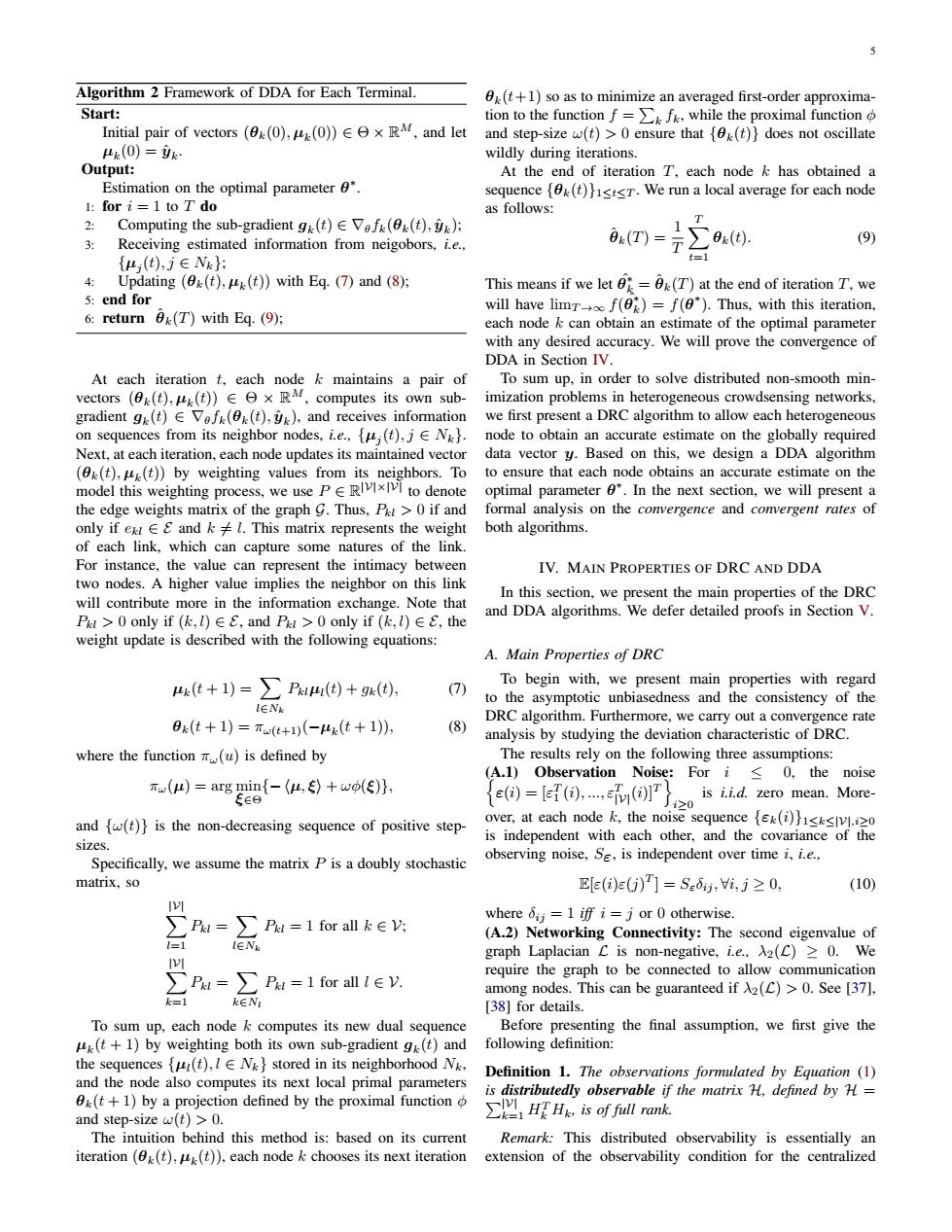
Algorithm 2 Framework of DDA for Each Terminal. 0(t+1)so as to minimize an averaged first-order approxima- Start: tion to the function f=kfk,while the proximal function Initial pair of vectors ((0),())ex RM,and let and step-size w(t)>0 ensure that (t)}does not oscillate Lk(0)= wildly during iterations. Output: At the end of iteration T,each node k has obtained a Estimation on the optimal parameter 6". sequence [(t))istsT.We run a local average for each node 1:for i=1 to T do as follows: 2: Computing the sub-gradient g(t)E Vofk ((t),) T 3: Receiving estimated information from neigobors,i.e., 0x(T)=T (9) {μ(t),j∈Nk t=l 4: Updating (x(t),u(t))with Eq.(7)and (8); This means if we let 0=(T)at the end of iteration T,we 5:end for will have limrof()=f(0).Thus,with this iteration, 6:return 0x(T)with Eq.(9); each node k can obtain an estimate of the optimal parameter with any desired accuracy.We will prove the convergence of DDA in Section IV. At each iteration t,each node k maintains a pair of To sum up,in order to solve distributed non-smooth min- vectors(Bk(t),hk()∈日×R,computes its own sub- imization problems in heterogeneous crowdsensing networks, gradient g(t)E Vofk((t),i).and receives information we first present a DRC algorithm to allow each heterogeneous on sequences from its neighbor nodes,i.e..u,(t),j N).node to obtain an accurate estimate on the globally required Next,at each iteration,each node updates its maintained vector data vector y.Based on this,we design a DDA algorithm (0k(t),u(t))by weighting values from its neighbors.To to ensure that each node obtains an accurate estimate on the model this weighting process,we use PRvlx to denote optimal parameter 0".In the next section,we will present a the edge weights matrix of the graph g.Thus,P>0 if and formal analysis on the convergence and convergent rates of only if ekt∈￡andk≠l.This matrix represents the weight both algorithms. of each link,which can capture some natures of the link. For instance,the value can represent the intimacy between IV.MAIN PROPERTIES OF DRC AND DDA two nodes.A higher value implies the neighbor on this link will contribute more in the information exchange.Note that In this section,we present the main properties of the DRC P >0 only if (1)EE,and Pk >0 only if (k,l)EE,the and DDA algorithms.We defer detailed proofs in Section V. weight update is described with the following equations: A.Main Properties of DRC k(t+1)=∑P()+9(), (7) To begin with,we present main properties with regard to the asymptotic unbiasedness and the consistency of the IENk 0k(t+1)=Twt+1)(-k(t+1): (8) DRC algorithm.Furthermore,we carry out a convergence rate analysis by studying the deviation characteristic of DRC. where the function (u)is defined by The results rely on the following three assumptions: (A.1)Observation Noise:For i<0,the noise πw(μ)=arg min{-(μ，)+w(ξ)} E∈e 间=间，P}.2i is i.i.d.zero mean.More- and f(t)}is the non-decreasing sequence of positive step- over,at each node k,the noise sequence ek(i)sk.zo is independent with each other,and the covariance of the sizes. Specifically,we assume the matrix P is a doubly stochastic observing noise,Se,is independent over time i,i.e., matrix,so E[e()e0)T]=Sed,i,j≥0， (10) 以 ∑Pk=Pu=1 for all: where 6ij=1 iff i=j or 0 otherwise. (A.2)Networking Connectivity:The second eigenvalue of l=1 IENk graph Laplacian C is non-negative,i.e.,A2(C)>0.We ∑Pa=∑Pa=1 for all v. require the graph to be connected to allow communication among nodes.This can be guaranteed if A2(C)>0.See [37]. k=1 k∈N [38]for details. To sum up,each node k computes its new dual sequence Before presenting the final assumption,we first give the (t+1)by weighting both its own sub-gradient g(t)and following definition: the sequences {u(t),IE N}stored in its neighborhood N. Definition 1.The observations formulated by Equation (1) and the node also computes its next local primal parameters is distributedly observable if the matrix H.defined by H= (t+1)by a projection defined by the proximal function and step-size w(t)>0. ∑1HgH,iso时full rank. The intuition behind this method is:based on its current Remark:This distributed observability is essentially an iteration ((t),(t)),each node k chooses its next iteration extension of the observability condition for the centralized5 Algorithm 2 Framework of DDA for Each Terminal. Start: Initial pair of vectors (θk(0), µk (0)) ∈ Θ × RM, and let µk (0) = yˆk . Output: Estimation on the optimal parameter θ ∗ . 1: for i = 1 to T do 2: Computing the sub-gradient gk (t) ∈ ∇θfk(θk(t), yˆk ); 3: Receiving estimated information from neigobors, i.e., {µj (t), j ∈ Nk}; 4: Updating (θk(t), µk (t)) with Eq. (7) and (8); 5: end for 6: return θˆ k(T) with Eq. (9); At each iteration t, each node k maintains a pair of vectors (θk(t), µk (t)) ∈ Θ × RM, computes its own sub￾gradient gk (t) ∈ ∇θfk(θk(t), yˆk ), and receives information on sequences from its neighbor nodes, i.e., {µj (t), j ∈ Nk}. Next, at each iteration, each node updates its maintained vector (θk(t), µk (t)) by weighting values from its neighbors. To model this weighting process, we use P ∈ R |V|×|V| to denote the edge weights matrix of the graph G. Thus, Pkl > 0 if and only if ekl ∈ E and k ̸= l. This matrix represents the weight of each link, which can capture some natures of the link. For instance, the value can represent the intimacy between two nodes. A higher value implies the neighbor on this link will contribute more in the information exchange. Note that Pkl > 0 only if (k, l) ∈ E, and Pkl > 0 only if (k, l) ∈ E, the weight update is described with the following equations: µk (t + 1) = ∑ l∈Nk Pklµl (t) + gk(t), (7) θk(t + 1) = πω(t+1)(−µk (t + 1)), (8) where the function πω(u) is defined by πω(µ) = arg min ξ∈Θ {− ⟨µ, ξ⟩ + ωϕ(ξ)}, and {ω(t)} is the non-decreasing sequence of positive step￾sizes. Specifically, we assume the matrix P is a doubly stochastic matrix, so ∑ |V| l=1 Pkl = ∑ l∈Nk Pkl = 1 for all k ∈ V; ∑ |V| k=1 Pkl = ∑ k∈Nl Pkl = 1 for all l ∈ V. To sum up, each node k computes its new dual sequence µk (t + 1) by weighting both its own sub-gradient gk (t) and the sequences {µl (t), l ∈ Nk} stored in its neighborhood Nk, and the node also computes its next local primal parameters θk(t + 1) by a projection defined by the proximal function ϕ and step-size ω(t) > 0. The intuition behind this method is: based on its current iteration (θk(t), µk (t)), each node k chooses its next iteration θk(t+1) so as to minimize an averaged first-order approxima￾tion to the function f = ∑ k fk, while the proximal function ϕ and step-size ω(t) > 0 ensure that {θk(t)} does not oscillate wildly during iterations. At the end of iteration T, each node k has obtained a sequence {θk(t)}1≤t≤T . We run a local average for each node as follows: θˆ k(T) = 1 T ∑ T t=1 θk(t). (9) This means if we let ˆθ ∗ k = θˆ k(T) at the end of iteration T, we will have limT→∞ f( ˆθ ∗ k ) = f(θ ∗ ). Thus, with this iteration, each node k can obtain an estimate of the optimal parameter with any desired accuracy. We will prove the convergence of DDA in Section IV. To sum up, in order to solve distributed non-smooth min￾imization problems in heterogeneous crowdsensing networks, we first present a DRC algorithm to allow each heterogeneous node to obtain an accurate estimate on the globally required data vector y. Based on this, we design a DDA algorithm to ensure that each node obtains an accurate estimate on the optimal parameter θ ∗ . In the next section, we will present a formal analysis on the convergence and convergent rates of both algorithms. IV. MAIN PROPERTIES OF DRC AND DDA In this section, we present the main properties of the DRC and DDA algorithms. We defer detailed proofs in Section V. A. Main Properties of DRC To begin with, we present main properties with regard to the asymptotic unbiasedness and the consistency of the DRC algorithm. Furthermore, we carry out a convergence rate analysis by studying the deviation characteristic of DRC. The results rely on the following three assumptions: { (A.1) Observation Noise: For i ≤ 0, the noise ε(i) = [ε T 1 (i), ..., εT |V|(i)]T } i≥0 is i.i.d. zero mean. More￾over, at each node k, the noise sequence {εk(i)}1≤k≤|V|,i≥0 is independent with each other, and the covariance of the observing noise, Sε, is independent over time i, i.e., E[ε(i)ε(j) T ] = Sεδij , ∀i, j ≥ 0, (10) where δij = 1 iff i = j or 0 otherwise. (A.2) Networking Connectivity: The second eigenvalue of graph Laplacian L is non-negative, i.e., λ2(L) ≥ 0. We require the graph to be connected to allow communication among nodes. This can be guaranteed if λ2(L) > 0. See [37], [38] for details. Before presenting the final assumption, we first give the following definition: Definition 1. The observations formulated by Equation (1) is ∑ distributedly observable if the matrix H, defined by H = |V| k=1 HT k Hk, is of full rank. Remark: This distributed observability is essentially an extension of the observability condition for the centralized