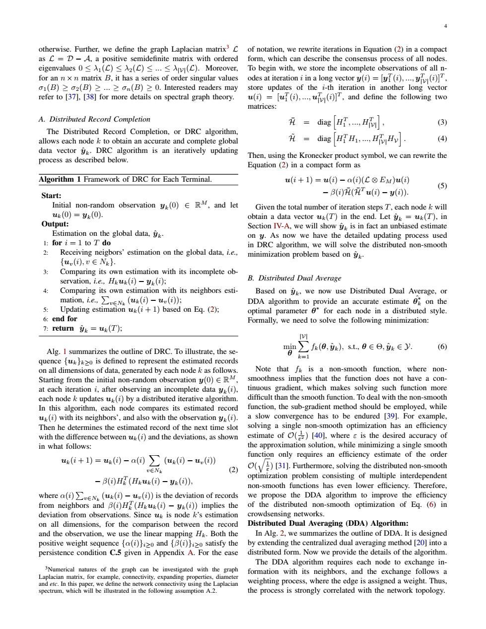
4 otherwise.Further,we define the graph Laplacian matrix3 C of notation,we rewrite iterations in Equation (2)in a compact as C=D-A,a positive semidefinite matrix with ordered form,which can describe the consensus process of all nodes eigenvalues0≤1(C)≤2(C)≤.≤vr(C).Moreover, To begin with.we store the incomplete observations of all n- for an n x n matrix B,it has a series of order singular values odes at iteration i in a long vector y()().( o1(B)≥2(B)≥.≥on(B)≥0.Interested readers may store updates of the i-th iteration in another long vector refer to [37].[38]for more details on spectral graph theory. u(i)=[uf(i),u()]T,and define the following two matrices: A.Distributed Record Completion =diag H..v, 孔 (3) The Distributed Record Completion,or DRC algorithm, allows each node k to obtain an accurate and complete global (4) data vectork.DRC algorithm is an iteratively updating process as described below. Then,using the Kronecker product symbol,we can rewrite the Equation (2)in a compact form as Algorithm 1 Framework of DRC for Each Terminal u(i+1)=u(i)-a(i)(C&EM)u(i) -B()i(严u()-y() (5) Start: Initial non-random observation yk(0)RM,and let Given the total number of iteration steps T,each node k will uk(0)=yx(0). obtain a data vector uk(T)in the end.Let ik uk(T),in Output: Section IV-A,we will show ik is in fact an unbiased estimate Estimation on the global data, on y.As now we have the detailed updating process used 1:for i=1 to T do in DRC algorithm,we will solve the distributed non-smooth 2: Receiving neigbors'estimation on the global data,i.e.. minimization problem based on yk. {u(i),v∈Nk 3: Comparing its own estimation with its incomplete ob- servation,i.e.,Hkuk(i)-yk(i): B.Distributed Dual Average Comparing its own estimation with its neighbors esti- Based on ik.we now use Distributed Dual Average,or mation,ie,∑uew(uk(）园-u.(i) DDA algorithm to provide an accurate estimate on the 5: Updating estimation uk(i+1)based on Eq.(2); optimal parameter 0*for each node in a distributed style. 6:end for Formally,we need to solve the following minimization: 7:return ik uk(T); (6) Alg.1 summarizes the outline of DRC.To illustrate,the se- min>f(0,9k),s.t,日∈日，9k∈y. quence [uk}o is defined to represent the estimated records k=1 on all dimensions of data,generated by each node k as follows. Note that f is a non-smooth function,where non- Starting from the initial non-random observation y(0)RM, smoothness implies that the function does not have a con- at each iteration i,after observing an incomplete data y(i), tinuous gradient,which makes solving such function more each node k updates uk(i)by a distributed iterative algorithm. difficult than the smooth function.To deal with the non-smooth In this algorithm,each node compares its estimated record function,the sub-gradient method should be employed,while uk(i)with its neighbors',and also with the observation y(i). a slow convergence has to be endured [39].For example, Then he determines the estimated record of the next time slot solving a single non-smooth optimization has an efficiency with the difference between uk(i)and the deviations,as shown estimate of ()[40],where is the desired accuracy of in what follows: the approximation solution,while minimizing a single smooth uk(位+1)=uk()-a()∑(u()-u() function only requires an efficiency estimate of the order ()[31].Furthermore,solving the distributed non-smooth -B(i)g (Hkuk(i)-yk(i)), optimization problem consisting of multiple interdependent non-smooth functions has even lower efficiency.Therefore, where a(i)vN(uk(i)-u(i))is the deviation of records we propose the DDA algorithm to improve the efficiency from neighbors and B(i)(Huk(i)-y(i))implies the of the distributed non-smooth optimization of Eq.(6)in deviation from observations.Since uk is node k's estimation crowdsensing networks. on all dimensions,for the comparison between the record Distributed Dual Averaging(DDA)Algorithm: and the observation,we use the linear mapping Hi.Both the In Alg.2,we summarizes the outline of DDA.It is designed positive weight sequence fa(i)}izo and [B(i)}izo satisfy the by extending the centralized dual averaging method [20]into a persistence condition C.5 given in Appendix A.For the ease distributed form.Now we provide the details of the algorithm. The DDA algorithm requires each node to exchange in- 3Numerical natures of the graph can be investigated with the graph formation with its neighbors,and the exchange follows a Laplacian matrix,for example,connectivity,expanding properties,diameter and etc.In this paper,we define the network connectivity using the Laplacian weighting process,where the edge is assigned a weight.Thus, spectrum,which will be illustrated in the following assumption A.2. the process is strongly correlated with the network topology4 otherwise. Further, we define the graph Laplacian matrix3 L as L = D − A, a positive semidefinite matrix with ordered eigenvalues 0 ≤ λ1(L) ≤ λ2(L) ≤ ... ≤ λ|V|(L). Moreover, for an n × n matrix B, it has a series of order singular values σ1(B) ≥ σ2(B) ≥ ... ≥ σn(B) ≥ 0. Interested readers may refer to [37], [38] for more details on spectral graph theory. A. Distributed Record Completion The Distributed Record Completion, or DRC algorithm, allows each node k to obtain an accurate and complete global data vector yˆk . DRC algorithm is an iteratively updating process as described below. Algorithm 1 Framework of DRC for Each Terminal. Start: Initial non-random observation yk (0) ∈ RM, and let uk(0) = yk (0). Output: Estimation on the global data, yˆk . 1: for i = 1 to T do 2: Receiving neigbors’ estimation on the global data, i.e., {uv(i), v ∈ Nk}. 3: Comparing its own estimation with its incomplete ob￾servation, i.e., Hkuk(i) − yk (i); 4: Comparing its own estimation with its neighbors esti￾mation, i.e., ∑ v∈Nk (uk(i) − uv(i)); 5: Updating estimation uk(i + 1) based on Eq. (2); 6: end for 7: return yˆk = uk(T); Alg. 1 summarizes the outline of DRC. To illustrate, the se￾quence {uk}k≥0 is defined to represent the estimated records on all dimensions of data, generated by each node k as follows. Starting from the initial non-random observation y(0) ∈ RM, at each iteration i, after observing an incomplete data yk (i), each node k updates uk(i) by a distributed iterative algorithm. In this algorithm, each node compares its estimated record uk(i) with its neighbors’, and also with the observation yk (i). Then he determines the estimated record of the next time slot with the difference between uk(i) and the deviations, as shown in what follows: uk(i + 1) = uk(i) − α(i) ∑ v∈Nk (uk(i) − uv(i)) − β(i)HT k (Hkuk(i) − yk (i)), (2) where α(i) ∑ v∈Nk (uk(i) − uv(i)) is the deviation of records from neighbors and β(i)HT k (Hkuk(i) − yk (i)) implies the deviation from observations. Since uk is node k’s estimation on all dimensions, for the comparison between the record and the observation, we use the linear mapping Hk. Both the positive weight sequence {α(i)}i≥0 and {β(i)}i≥0 satisfy the persistence condition C.5 given in Appendix A. For the ease 3Numerical natures of the graph can be investigated with the graph Laplacian matrix, for example, connectivity, expanding properties, diameter and etc. In this paper, we define the network connectivity using the Laplacian spectrum, which will be illustrated in the following assumption A.2. of notation, we rewrite iterations in Equation (2) in a compact form, which can describe the consensus process of all nodes. To begin with, we store the incomplete observations of all n￾odes at iteration i in a long vector y(i) = [y T 1 (i), ..., y T |V|(i)]T , store updates of the i-th iteration in another long vector u(i) = [u T 1 (i), ..., u T |V|(i)]T , and define the following two matrices: H¯ = diag [ HT 1 , ..., HT |V|] , (3) H˜ = diag [ HT 1 H1, ..., HT |V|HV ] . (4) Then, using the Kronecker product symbol, we can rewrite the Equation (2) in a compact form as u(i + 1) = u(i) − α(i)(L ⊗ EM)u(i) − β(i)H¯(H¯Tu(i) − y(i)). (5) Given the total number of iteration steps T, each node k will obtain a data vector uk(T) in the end. Let yˆk = uk(T), in Section IV-A, we will show yˆk is in fact an unbiased estimate on y. As now we have the detailed updating process used in DRC algorithm, we will solve the distributed non-smooth minimization problem based on yˆk . B. Distributed Dual Average Based on yˆk , we now use Distributed Dual Average, or DDA algorithm to provide an accurate estimate ˆθ ∗ k on the optimal parameter θ ∗ for each node in a distributed style. Formally, we need to solve the following minimization: min θ ∑ |V| k=1 fk(θ, yˆk ), s.t., θ ∈ Θ, yˆk ∈ Y. (6) Note that fk is a non-smooth function, where non￾smoothness implies that the function does not have a con￾tinuous gradient, which makes solving such function more difficult than the smooth function. To deal with the non-smooth function, the sub-gradient method should be employed, while a slow convergence has to be endured [39]. For example, solving a single non-smooth optimization has an efficiency estimate of O( 1 ε 2 ) [40], where ε is the desired accuracy of the approximation solution, while minimizing a single smooth function only requires an efficiency estimate of the order O( √ 1 ε ) [31]. Furthermore, solving the distributed non-smooth optimization problem consisting of multiple interdependent non-smooth functions has even lower efficiency. Therefore, we propose the DDA algorithm to improve the efficiency of the distributed non-smooth optimization of Eq. (6) in crowdsensing networks. Distributed Dual Averaging (DDA) Algorithm: In Alg. 2, we summarizes the outline of DDA. It is designed by extending the centralized dual averaging method [20] into a distributed form. Now we provide the details of the algorithm. The DDA algorithm requires each node to exchange in￾formation with its neighbors, and the exchange follows a weighting process, where the edge is assigned a weight. Thus, the process is strongly correlated with the network topology