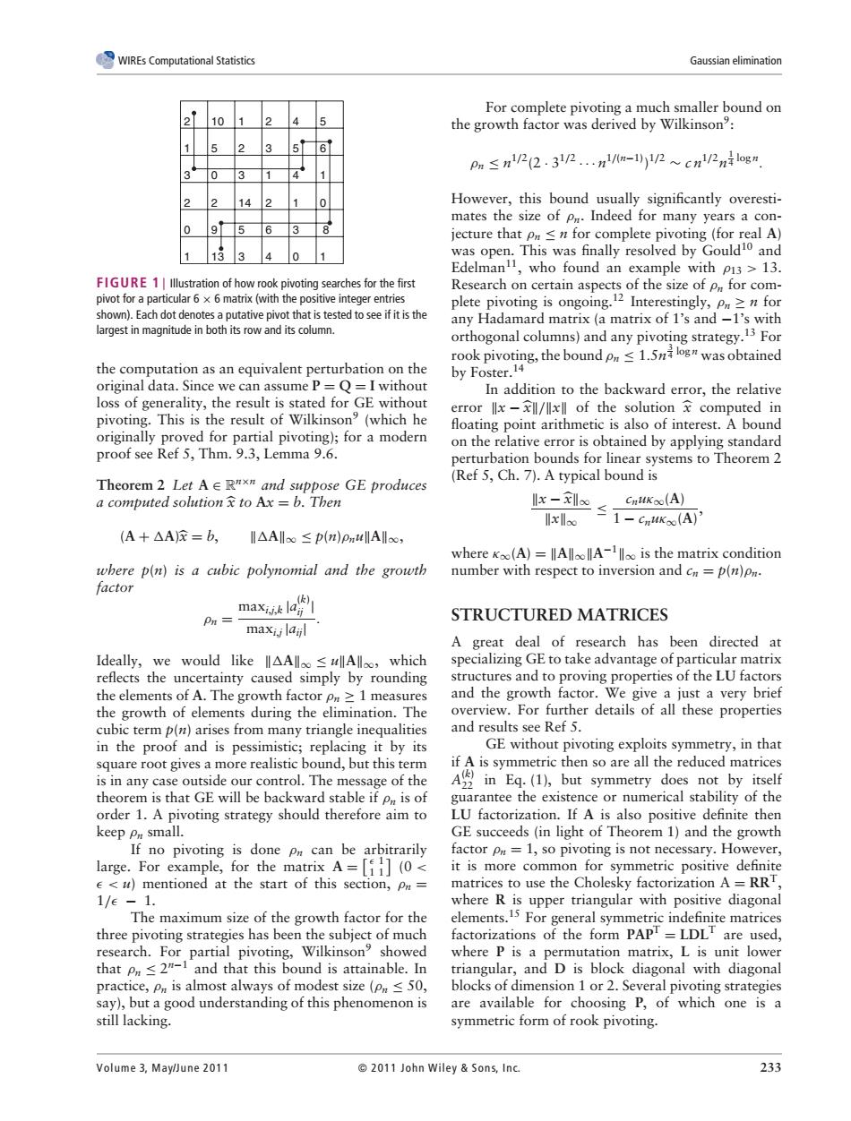
WIREs Computational Statistic the o Fo 。，， Pa≤n1/22.3p…n2m-)2nog 14210 However,this bound usually significantly overesti- 95638 133401 complete pivot who found nx ho).putative pivot that istested plere pivotineof the sire of for Interes largest in magnitude in both its row and its column original nce we ca assume. In addition to the backward error,the relative This is the r :is alsc of int proof see Ref 5,Thm.9.3,Lemma 9.6. Theorem 2 Let A E R"xm and su e GE produces (Ref 5,Ch.).Aypical bound a computed solution to Ax=b.Then llx-3 (A) (A+△A=b, I△A≤p)Allo (A) where (A)=AllA-l is the matrix condition where p(n)is a cubic polynomial and the growth number with respect to inversion and c=p(n) factor maxz la) Pn= STRUCTURED MATRICES directed structures and to proving properties of the LU factor the elements of a The growth facto 1 measure and the growth fa ctor. We give a just a very brief the growth of elements during the elimination.The rview.For arther details of all these properties cub term p(n)arises from many triangle inequalitie and r in the pro etry.in tha if A is symmetric then so are all the reduced matrice is in any case outside our control.The message of the A in Eq.(1),but symmetry does not by itself theorem is that GE will be backward stable if is of order 1.A facto A 15 1 so it is more comm on for symmetric positive definit u)mentioned at the start of this section,p= Cholesky RR re upper triangular e maxi thre actor fo research.For partial ing.Wilkinson?showed where P is a nutation matrix,L is unit lower that p≤2 nd that this l bound is attainable.In ts1ZePm≤ 0r2. ng o P.of of Volume 3.Maylune 201 2011 John wiley sons.Inc 233WIREs Computational Statistics Gaussian elimination 2 1 3 2 0 1 10 5 0 2 9 13 1 2 3 14 5 3 2 3 1 2 6 4 4 5 4 1 3 0 5 6 1 0 8 1 FIGURE 1 | Illustration of how rook pivoting searches for the first pivot for a particular 6 × 6 matrix (with the positive integer entries shown). Each dot denotes a putative pivot that is tested to see if it is the largest in magnitude in both its row and its column. the computation as an equivalent perturbation on the original data. Since we can assume P = Q = I without loss of generality, the result is stated for GE without pivoting. This is the result of Wilkinson9 (which he originally proved for partial pivoting); for a modern proof see Ref 5, Thm. 9.3, Lemma 9.6. Theorem 2 Let A ∈ Rn×n and suppose GE produces a computed solution x to Ax = b. Then (A + A)x = b, A∞ ≤ p(n)ρnuA∞, where p(n) is a cubic polynomial and the growth factor ρn = maxi,j,k |a (k) ij | maxi,j |aij| . Ideally, we would like A∞ ≤ uA∞, which reflects the uncertainty caused simply by rounding the elements of A. The growth factor ρn ≥ 1 measures the growth of elements during the elimination. The cubic term p(n) arises from many triangle inequalities in the proof and is pessimistic; replacing it by its square root gives a more realistic bound, but this term is in any case outside our control. The message of the theorem is that GE will be backward stable if ρn is of order 1. A pivoting strategy should therefore aim to keep ρn small. If no pivoting is done ρn can be arbitrarily large. For example, for the matrix A =  1 1 1  (0 < < u) mentioned at the start of this section, ρn = 1/ − 1. The maximum size of the growth factor for the three pivoting strategies has been the subject of much research. For partial pivoting, Wilkinson9 showed that ρn ≤ 2n−1 and that this bound is attainable. In practice, ρn is almost always of modest size (ρn ≤ 50, say), but a good understanding of this phenomenon is still lacking. For complete pivoting a much smaller bound on the growth factor was derived by Wilkinson9: ρn ≤ n1/2(2 · 31/2 ··· n1/(n−1)) 1/2 ∼ c n1/2n 1 4 log n. However, this bound usually significantly overesti￾mates the size of ρn. Indeed for many years a con￾jecture that ρn ≤ n for complete pivoting (for real A) was open. This was finally resolved by Gould10 and Edelman11, who found an example with ρ13 > 13. Research on certain aspects of the size of ρn for com￾plete pivoting is ongoing.12 Interestingly, ρn ≥ n for any Hadamard matrix (a matrix of 1’s and −1’s with orthogonal columns) and any pivoting strategy.13 For rook pivoting, the bound ρn ≤ 1.5n 3 4 log n was obtained by Foster.14 In addition to the backward error, the relative error x −x/x of the solution x computed in floating point arithmetic is also of interest. A bound on the relative error is obtained by applying standard perturbation bounds for linear systems to Theorem 2 (Ref 5, Ch. 7). A typical bound is x −x∞ x∞ ≤ cnuκ∞(A) 1 − cnuκ∞(A) , where κ∞(A) = A∞A−1∞ is the matrix condition number with respect to inversion and cn = p(n)ρn. STRUCTURED MATRICES A great deal of research has been directed at specializing GE to take advantage of particular matrix structures and to proving properties of the LU factors and the growth factor. We give a just a very brief overview. For further details of all these properties and results see Ref 5. GE without pivoting exploits symmetry, in that if A is symmetric then so are all the reduced matrices A(k) 22 in Eq. (1), but symmetry does not by itself guarantee the existence or numerical stability of the LU factorization. If A is also positive definite then GE succeeds (in light of Theorem 1) and the growth factor ρn = 1, so pivoting is not necessary. However, it is more common for symmetric positive definite matrices to use the Cholesky factorization A = RRT, where R is upper triangular with positive diagonal elements.15 For general symmetric indefinite matrices factorizations of the form PAPT = LDLT are used, where P is a permutation matrix, L is unit lower triangular, and D is block diagonal with diagonal blocks of dimension 1 or 2. Several pivoting strategies are available for choosing P, of which one is a symmetric form of rook pivoting. Volume 3, May/June 2011  2011 John Wiley & Son s, In c. 233