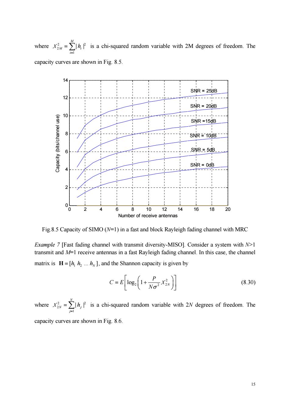
where is a chi-squared random variable with 2M degrees of freedom.The capacity curves are shown in Fig.8.5 SNR 25HB 72 SNR=20dB SNR =154B SNR 100B- SNR=508_ SNR=O电 6 8 10 14 16 18 20 Number of receive antennas Fig8.5 Capacity of SIMO(N=1)in a fast and block Rayleigh fading channel with MRC Example 7 [Fast fading channel with transmit diversity-MISO].Consider a system with N>I transmit and M1 receive antennas in a fast Rayleigh fading channel.In this case,the channel matrix is H=[.and the Shannon capacity is given by c=e〔石】 (8.30) where is a chi-squared random variable with 2N degrees of freedom.The capacity curves are shown in Fig.8.6. 15 15 where 2 2 2 1 | | M M i i h  X   is a chi-squared random variable with 2M degrees of freedom. The capacity curves are shown in Fig. 8.5. 0 2 4 6 8 10 12 14 16 18 20 0 2 4 6 8 10 12 14 Number of receive antennas Capacity (bits/channel use) SNR = 0dB SNR = 5dB SNR = 10dB SNR =15dB SNR = 20dB SNR = 25dB Fig.8.5 Capacity of SIMO (N=1) in a fast and block Rayleigh fading channel with MRC Example 7 [Fast fading channel with transmit diversity-MISO]. Consider a system with N>1 transmit and M=1 receive antennas in a fast Rayleigh fading channel. In this case, the channel matrix is 1 2 [ . ] N H  hh h , and the Shannon capacity is given by 2 2 2 2 log 1 N P C E N            X (8.30) where 2 2 2 1 | | N N j j h  X   is a chi-squared random variable with 2N degrees of freedom. The capacity curves are shown in Fig. 8.6