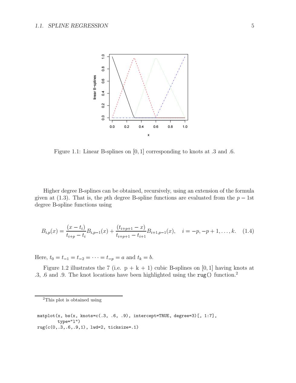
1.1.SPLINE REGRESSION 8 8 0.0 0.2 0.40.6 0.81.0 Figure 1.1:Linear B-splines on 0,1]corresponding to knots at.3 and.6. Higher degree B-splines can be obtained,recursively,using an extension of the formula given at(1.3).That is,the pth degree B-spline functions are evaluated from the p-lst degree B-spline functions using B回=B-回+A-1e.i=-n-p+1,k1到 titp-ti titpt1-titl Here,to =t_1=t_2=...=t-p a and t=b. Figure 1.2 illustrates the 7 (i.e.p +k +1)cubic B-splines on [0,1]having knots at .3,.6 and.9.The knot locations have been highlighted using the rug()function.? 2This plot is obtained using matplot(x,bs(x,knots=c(.3,.6,.9),intercept=TRUE,degree=3)[,1:7], type="1") rug(c(0,.3,.6,.9,1),1wd=2,ticksize=.1)1.1. SPLINE REGRESSION 5 0.0 0.2 0.4 0.6 0.8 1.0 0.0 0.2 0.4 0.6 0.8 1.0 x linear B−splines Figure 1.1: Linear B-splines on [0, 1] corresponding to knots at .3 and .6. Higher degree B-splines can be obtained, recursively, using an extension of the formula given at (1.3). That is, the pth degree B-spline functions are evaluated from the p − 1st degree B-spline functions using Bi,p(x) = (x − ti) ti+p − ti Bi,p−1(x) + (ti+p+1 − x) ti+p+1 − ti+1 Bi+1,p−1(x), i = −p, −p + 1, . . . , k. (1.4) Here, t0 = t−1 = t−2 = · · · = t−p = a and tk = b. Figure 1.2 illustrates the 7 (i.e. p + k + 1) cubic B-splines on [0, 1] having knots at .3, .6 and .9. The knot locations have been highlighted using the rug() function.2 2This plot is obtained using matplot(x, bs(x, knots=c(.3, .6, .9), intercept=TRUE, degree=3)[, 1:7], type="l") rug(c(0,.3,.6,.9,1), lwd=2, ticksize=.1)