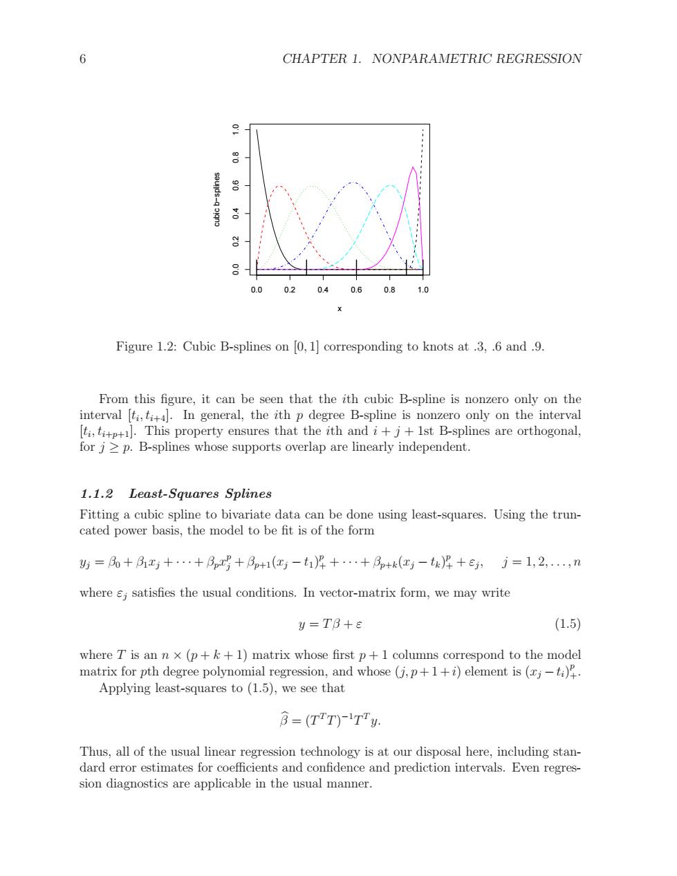
6 CHAPTER 1.NONPARAMETRIC REGRESSION 0.0 0.2 0.4 0.6 0.8 1.0 Figure 1.2:Cubic B-splines on [0,1]corresponding to knots at.3,.6 and.9. From this figure,it can be seen that the ith cubic B-spline is nonzero only on the interval [ti,tit4.In general,the ith p degree B-spline is nonzero only on the interval [ti,tp].This property ensures that the ith and i+j+1st B-splines are orthogonal, for j>p.B-splines whose supports overlap are linearly independent. 1.1.2 Least-Squares Splines Fitting a cubic spline to bivariate data can be done using least-squares.Using the trun- cated power basis,the model to be fit is of the form 斯=0+月x+…+月n+月+1（红-t岸+…+月+k(c-t)4+e,j=1,2,,n where s;satisfies the usual conditions.In vector-matrix form,we may write y=TB+E (1.5) where T is an nx(p+k+1)matrix whose first p+1 columns correspond to the model matrix for pth degree polynomial regression,and whose (j,p+1+i)element is (j) Applying least-squares to (1.5),we see that 3=(TT)-1Ty. Thus,all of the usual linear regression technology is at our disposal here,including stan- dard error estimates for coefficients and confidence and prediction intervals.Even regres- sion diagnostics are applicable in the usual manner.6 CHAPTER 1. NONPARAMETRIC REGRESSION 0.0 0.2 0.4 0.6 0.8 1.0 0.0 0.2 0.4 0.6 0.8 1.0 x cubic b−splines Figure 1.2: Cubic B-splines on [0, 1] corresponding to knots at .3, .6 and .9. From this figure, it can be seen that the ith cubic B-spline is nonzero only on the interval [ti , ti+4]. In general, the ith p degree B-spline is nonzero only on the interval [ti , ti+p+1]. This property ensures that the ith and i + j + 1st B-splines are orthogonal, for j ≥ p. B-splines whose supports overlap are linearly independent. 1.1.2 Least-Squares Splines Fitting a cubic spline to bivariate data can be done using least-squares. Using the trun￾cated power basis, the model to be fit is of the form yj = β0 + β1xj + · · · + βpx p j + βp+1(xj − t1) p + + · · · + βp+k(xj − tk) p + + εj , j = 1, 2, . . . , n where εj satisfies the usual conditions. In vector-matrix form, we may write y = T β + ε (1.5) where T is an n × (p + k + 1) matrix whose first p + 1 columns correspond to the model matrix for pth degree polynomial regression, and whose (j, p+ 1 +i) element is (xj −ti) p +. Applying least-squares to (1.5), we see that βb = (T T T) −1T T y. Thus, all of the usual linear regression technology is at our disposal here, including stan￾dard error estimates for coefficients and confidence and prediction intervals. Even regres￾sion diagnostics are applicable in the usual manner