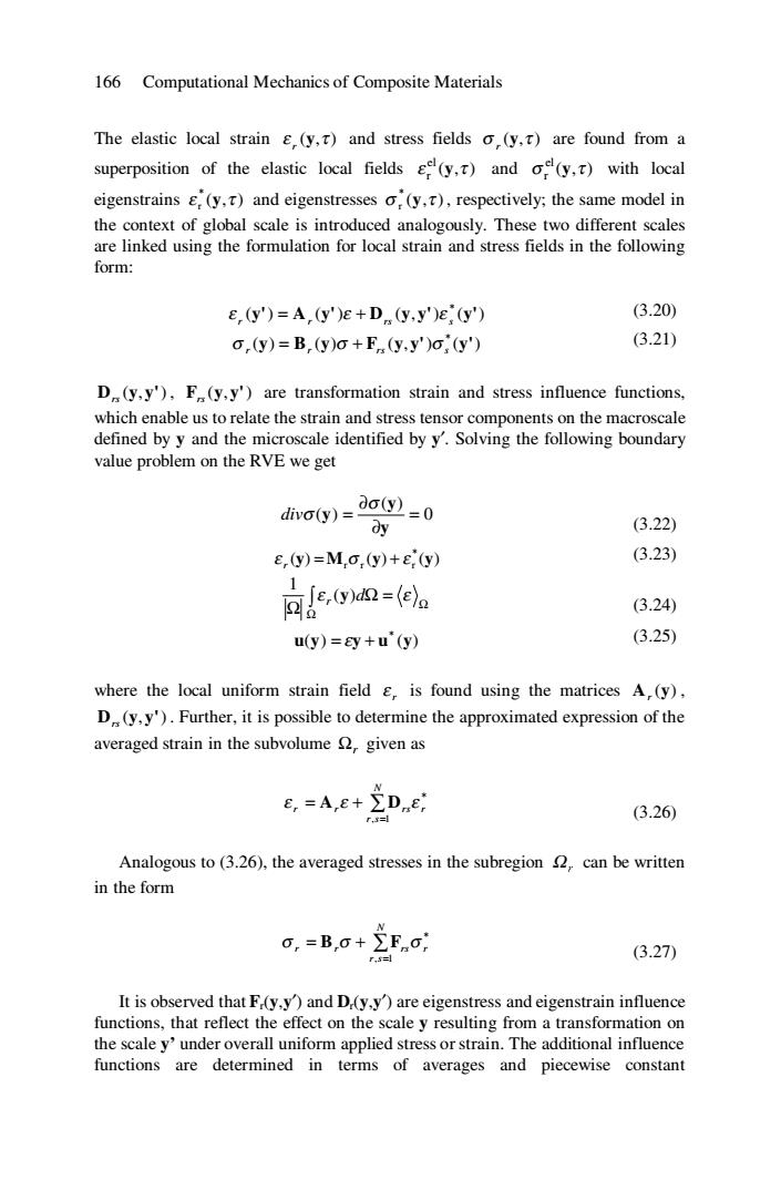
166 Computational Mechanics of Composite Materials The elastic local strain (y,t)and stress fields o(y,t)are found from a superposition of the elastic local fields (y,)and of(y,)with local eigenstrains E,(y,T)and eigenstresses o,(y,t),respectively;the same model in the context of global scale is introduced analogously.These two different scales are linked using the formulation for local strain and stress fields in the following form: e,(y')=A,(y')e+D.y,y')e(y') (3.20) o,(y)=B,(y)o+F.(y,y')o,(y') (3.21) D(y,y'),F(y,y')are transformation strain and stress influence functions, which enable us to relate the strain and stress tensor components on the macroscale defined by y and the microscale identified by y'.Solving the following boundary value problem on the RVE we get divo(y)= ∂o=0 ∂y (3.22) e,(y)=M,o,(y)+e(y) (3.23) 1 le,0an=ea (3.24) u(y)=ay+u"(y) (3.25) where the local uniform strain field E,is found using the matrices A,(y), D(y,y').Further,it is possible to determine the approximated expression of the averaged strain in the subvolume given as e,=A,e+∑D.e (3.26) Analogous to (3.26),the averaged stresses in the subregion 2,can be written in the form o,=B,0+∑Fn0i ,曰 (3.27) It is observed that F(y.y)and D.(y,y)are eigenstress and eigenstrain influence functions,that reflect the effect on the scale y resulting from a transformation on the scale y'under overall uniform applied stress or strain.The additional influence functions are determined in terms of averages and piecewise constant166 Computational Mechanics of Composite Materials The elastic local strain ) ε (y,τ r and stress fields ) σ (y,τ r are found from a superposition of the elastic local fields ) ( , el r ε y τ and ) ( , el r σ y τ with local eigenstrains ) ( , * r ε y τ and eigenstresses ) ( , * r σ y τ , respectively; the same model in the context of global scale is introduced analogously. These two different scales are linked using the formulation for local strain and stress fields in the following form: ( ) ( ) ( , ) ( ) * y' A y' D y y' y' r r rs s ε = ε + ε (3.20) ( ) ( ) ( , ) ( ) * y B y F y y' y' σ r = r σ + rs σ s (3.21) D (y, y') rs , ) F (y, y' rs are transformation strain and stress influence functions, which enable us to relate the strain and stress tensor components on the macroscale defined by y and the microscale identified by y′. Solving the following boundary value problem on the RVE we get 0 ( ) ( ) = ∂ ∂ = y y y σ divσ (3.22) ( ) ( ) ( ) * r r r ε y = M σ y + ε y r (3.23) ∫ Ω Ω Ω = Ω ε d ε r ( ) 1 y (3.24) ( ) ( ) * u y = εy + u y (3.25) where the local uniform strain field r ε is found using the matrices ) A (y r , D (y, y') rs . Further, it is possible to determine the approximated expression of the averaged strain in the subvolume Ωr given as ∑ = = + N r s r r rs r , 1 * ε A ε D ε (3.26) Analogous to (3.26), the averaged stresses in the subregion Ωr can be written in the form ∑ = = + N r s r r rs r , 1 * σ B σ F σ (3.27) It is observed that Fr(y,y′) and Dr(y,y′) are eigenstress and eigenstrain influence functions, that reflect the effect on the scale y resulting from a transformation on the scale y’ under overall uniform applied stress or strain. The additional influence functions are determined in terms of averages and piecewise constant