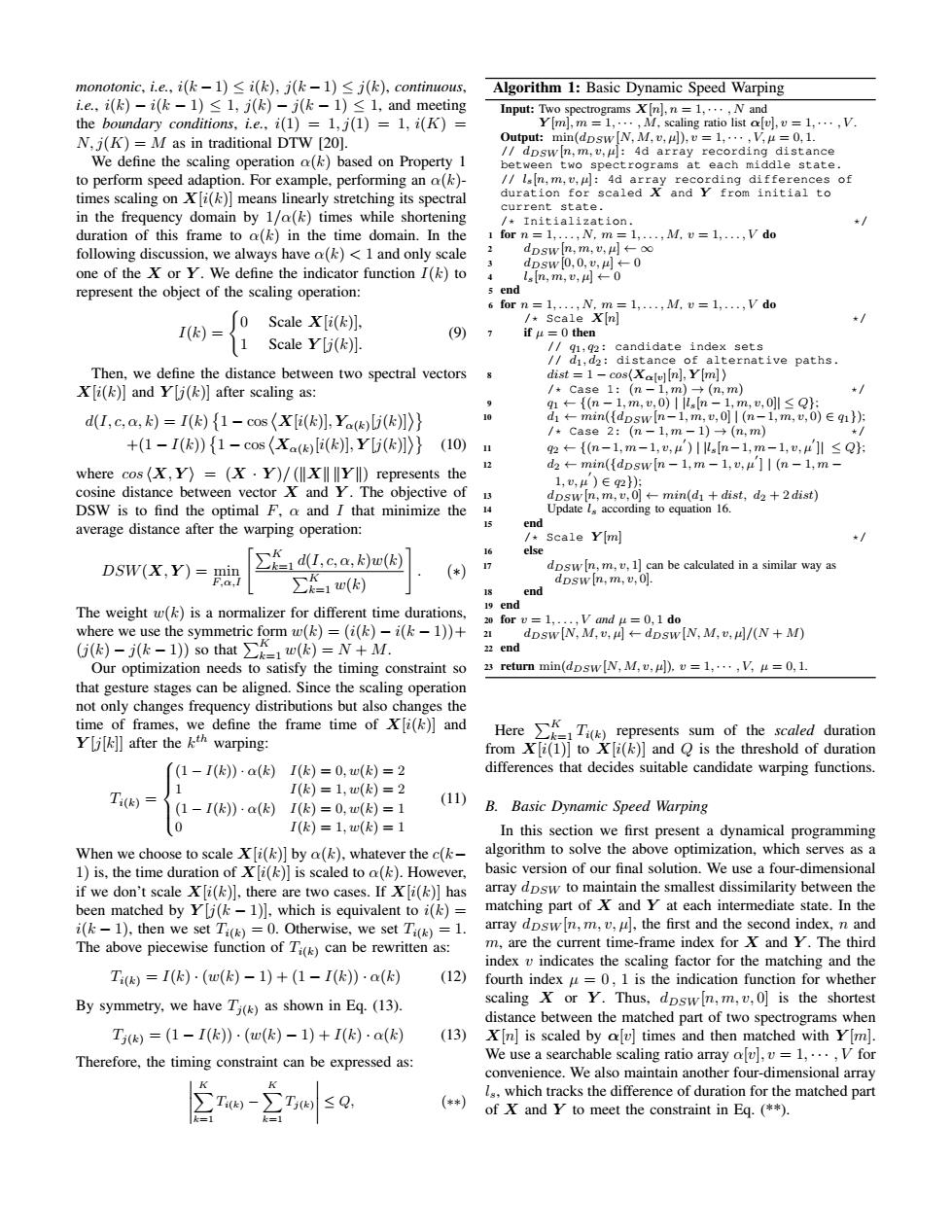
monotonic,i.e.,i(k-1)<i(k),j(k-1)<j(k),continuous, Algorithm 1:Basic Dynamic Speed Warping i.e.,i()-i(k-1)≤1，j(k)-j(k-1)≤1，and meeting Input:Two spectrograms Xnl,n 1,...,N and the boundary conditions,i.e.,i(1)=1,j(1)=1,i(K)= Y[m,m=1,·,M,scaling ratio list ou,v=l,·,V N,j(K)=M as in traditional DTW [20]. 0 utput::min(dDsw[N,M,u,4l,v=1,…,V,μ=0,1. /dpswn,m,v,u:4d array recording distance We define the scaling operation a(k)based on Property 1 between two spectrograms at each middle state. to perform speed adaption.For example,performing an a(k)- //Isn,m,v,ul:4d array recording differences of times scaling on X[i(k)]means linearly stretching its spectral duration for scaled X and Y from initial to current state. in the frequency domain by 1/a(k)times while shortening /Initialization. * duration of this frame to a(k)in the time domain.In the 1 for n 1,...,N,m =1,...,M.v =1,...,V do following discussion,we always have a(k)<1 and only scale 2 dpsw[n,m,u,l←o 3 dDsw0,0,u,4←0 one of the X or Y.We define the indicator function I(k)to 4 lsn,m,,4←0 represent the object of the scaling operation: 5 end 6 for n 1,...,N,m 1,...,M.v =1,...,V do 0 Scale x[i(k)], /scale Xn */ I()= (9) 7 1 Scale Y[i(k)] if=0 then //91,92:candidate index sets /d1,d2:distance of alternative paths. Then,we define the distance between two spectral vectors s dist =1-cos(Xalu]In],Y[m]) X[i(k)】andY[i(ke】after scaling as: /case 1:(n-1,m)(n,m) 9 9←{(n-1,m,u,0)|llsn-1,m,u,0l≤Q: d(I,c,a,k)=I(k){1-cos(x[i()],Ya(k() d←min({dpsw(n-1,m,u,0]I(n-1,m,u,0)∈91} /+case2:(n-1,m-1)→(n,m) ★ +(1-I(k)){1-cos(Xa(k)[i()],Y[j()] (10) 1 92←{(n-1,m-1,v,4)1lln-1,m-1,v,μ]l≤Q: where cos(X,Y)=(X.Y)/(represents the 12 d2←min({dpsw[n-1,m-1,u,μ]|(m-1,m- 1,0,4)∈92})： cosine distance between vector X and Y.The objective of dpsw [n,m,v,]+min(d1 dist,d2 +2dist) DSW is to find the optimal F.a and I that minimize the 14 Update ls according to equation 16. average distance after the warping operation: 15 end /Scale Y[ml */ else DSW(X,Y)=min ∑KdL,ca,k)u(因 17 dpsw[n,m,v,1]can be calculated in a similar way as ∑太1w(k (*) doswn,m,v,0. 18 end The weight w(k)is a normalizer for different time durations, 19 end 20 for v =1,...,V and u=0,1 do where we use the symmetric form w(k)=(i()-i(k-1))+ dpsw [N,M,v,udpsw [N,M,v,u]/(N+M) (j(k)-j(k-1))so that w(k)=N+M. 22 end Our optimization needs to satisfy the timing constraint so 23 return min(dpsw [N,M,v,u).v=1;...,V,=0,1. that gesture stages can be aligned.Since the scaling operation not only changes frequency distributions but also changes the time of frames,we define the frame time of X[i(k)]and Yk]]after the kth warping: HereT()represents sum of the scaled duration from X[i(1)]to X[i(k)]and Q is the threshold of duration (1-I()·a()I()=0,w()=2 differences that decides suitable candidate warping functions. 1 T)= I(k)=1,w()=2 (1-I()·a(k)I(k)=0,w()=1 (11) B.Basic Dynamic Speed Warping 0 I()=1,w(k)=1 In this section we first present a dynamical programming When we choose to scale Xi(k)]by a(k),whatever the c(k- algorithm to solve the above optimization,which serves as a 1)is,the time duration of X[i(k)]is scaled to a(k).However, basic version of our final solution.We use a four-dimensional if we don't scale X[i()],there are two cases.If X [i(k)]has array dpsw to maintain the smallest dissimilarity between the been matched by Y[j(k-1)],which is equivalent to i(k)= matching part of X and Y at each intermediate state.In the i(k-1).then we set Ti(k)=0.Otherwise,we set Ti(k)=1. array dpswn,m,v,u,the first and the second index,n and The above piecewise function of Ti(k)can be rewritten as: m,are the current time-frame index for X and Y.The third index v indicates the scaling factor for the matching and the T=I(k)·(w(E)-1)+(1-I()·a(E) (12) fourth index u=0,1 is the indication function for whether By symmetry,we have Ti(k)as shown in Eq.(13). scaling X or Y.Thus,dpsw[n,m,v,0]is the shortest distance between the matched part of two spectrograms when T)=(1-I(k)·(w()-1)+I()·a() (13) Xn is scaled by av]times and then matched with Y[m]. Therefore,the timing constraint can be expressed as: We use a searchable scaling ratio array av],v =1,...,V for convenience.We also maintain another four-dimensional array T-sQ. ls,which tracks the difference of duration for the matched part **) of X and Y to meet the constraint in Eq.(**)monotonic, i.e., i(k ￾ 1)  i(k), j(k ￾ 1)  j(k), continuous, i.e., i(k) ￾ i(k ￾ 1)  1, j(k) ￾ j(k ￾ 1)  1, and meeting the boundary conditions, i.e., i(1) = 1, j(1) = 1, i(K) = N, j(K) = M as in traditional DTW [20]. We define the scaling operation ↵(k) based on Property 1 to perform speed adaption. For example, performing an ↵(k)- times scaling on X[i(k)] means linearly stretching its spectral in the frequency domain by 1/↵(k) times while shortening duration of this frame to ↵(k) in the time domain. In the following discussion, we always have ↵(k) < 1 and only scale one of the X or Y . We define the indicator function I(k) to represent the object of the scaling operation: I(k) = ( 0 Scale X[i(k)], 1 Scale Y [j(k)]. (9) Then, we define the distance between two spectral vectors X[i(k)] and Y [j(k)] after scaling as: d(I, c, ↵, k) = I(k) ￾ 1 ￾ cos ⌦ X[i(k)],Y↵(k)[j(k)]↵ +(1 ￾ I(k)) ￾ 1 ￾ cos ⌦ X↵(k)[i(k)],Y [j(k)]↵ (10) where cos hX,Y i = (X · Y )/ (kXk kY k) represents the cosine distance between vector X and Y . The objective of DSW is to find the optimal F, ↵ and I that minimize the average distance after the warping operation: DSW(X,Y ) = min F,↵,I "PK k=1 d(I, c, ↵, k)w(k) PK k=1 w(k) # . (⇤) The weight w(k) is a normalizer for different time durations, where we use the symmetric form w(k)=(i(k) ￾ i(k ￾ 1))+ (j(k) ￾ j(k ￾ 1)) so that PK k=1 w(k) = N + M. Our optimization needs to satisfy the timing constraint so that gesture stages can be aligned. Since the scaling operation not only changes frequency distributions but also changes the time of frames, we define the frame time of X[i(k)] and Y [j[k]] after the kth warping: Ti(k) = 8 >>< >>: (1 ￾ I(k)) · ↵(k) I(k)=0, w(k)=2 1 I(k)=1, w(k)=2 (1 ￾ I(k)) · ↵(k) I(k)=0, w(k)=1 0 I(k)=1, w(k)=1 (11) When we choose to scale X[i(k)] by ↵(k), whatever the c(k￾ 1) is, the time duration of X[i(k)] is scaled to ↵(k). However, if we don’t scale X[i(k)], there are two cases. If X[i(k)] has been matched by Y [j(k ￾ 1)], which is equivalent to i(k) = i(k ￾ 1), then we set Ti(k) = 0. Otherwise, we set Ti(k) = 1. The above piecewise function of Ti(k) can be rewritten as: Ti(k) = I(k) · (w(k) ￾ 1) + (1 ￾ I(k)) · ↵(k) (12) By symmetry, we have Tj(k) as shown in Eq. (13). Tj(k) = (1 ￾ I(k)) · (w(k) ￾ 1) + I(k) · ↵(k) (13) Therefore, the timing constraint can be expressed as: ￾ ￾ ￾ ￾ ￾ XK k=1 Ti(k) ￾XK k=1 Tj(k) ￾ ￾ ￾ ￾ ￾  Q, (⇤⇤) Algorithm 1: Basic Dynamic Speed Warping Input: Two spectrograms X[n], n = 1, ··· , N and Y [m], m = 1, ··· , M, scaling ratio list ↵[v], v = 1, ··· , V . Output: min(dDSW [N,M, v, µ]), v = 1, ··· ,V,µ = 0, 1. // dDSW [n, m, v, µ]: 4d array recording distance between two spectrograms at each middle state. // ls[n, m, v, µ]: 4d array recording differences of duration for scaled X and Y from initial to current state. /* Initialization. */ 1 for n = 1,...,N, m = 1,...,M, v = 1,...,V do 2 dDSW [n, m, v, µ] 1 3 dDSW [0, 0, v, µ] 0 4 ls[n, m, v, µ] 0 5 end 6 for n = 1,...,N, m = 1,...,M, v = 1,...,V do /* Scale X[n] */ 7 if µ = 0 then // q1, q2: candidate index sets // d1, d2: distance of alternative paths. 8 dist = 1 ￾ coshX↵[v][n], Y [m] i /* Case 1: (n ￾ 1, m) ! (n, m) */ 9 q1 {(n ￾ 1, m, v, 0) | |ls[n ￾ 1, m, v, 0]|  Q}; 10 d1 min({dDSW [n￾1, m, v, 0] | (n￾1, m, v, 0) 2 q1}); /* Case 2: (n ￾ 1, m ￾ 1) ! (n, m) */ 11 q2 {(n￾1, m￾1, v, µ0 ) | |ls[n￾1, m￾1, v, µ0 ]|  Q}; 12 d2 min({dDSW [n ￾ 1, m ￾ 1, v, µ0 ] | (n ￾ 1, m ￾ 1, v, µ0 ) 2 q2}); 13 dDSW [n, m, v, 0] min(d1 + dist, d2 + 2 dist) 14 Update ls according to equation 16. 15 end /* Scale Y [m] */ 16 else 17 dDSW [n, m, v, 1] can be calculated in a similar way as dDSW [n, m, v, 0]. 18 end 19 end 20 for v = 1,...,V and µ = 0, 1 do 21 dDSW [N,M, v, µ] dDSW [N,M, v, µ]/(N + M) 22 end 23 return min(dDSW [N,M, v, µ]), v = 1, ··· ,V, µ = 0, 1. Here PK k=1 Ti(k) represents sum of the scaled duration from X[i(1)] to X[i(k)] and Q is the threshold of duration differences that decides suitable candidate warping functions. B. Basic Dynamic Speed Warping In this section we first present a dynamical programming algorithm to solve the above optimization, which serves as a basic version of our final solution. We use a four-dimensional array dDSW to maintain the smallest dissimilarity between the matching part of X and Y at each intermediate state. In the array dDSW [n, m, v, µ], the first and the second index, n and m, are the current time-frame index for X and Y . The third index v indicates the scaling factor for the matching and the fourth index µ = 0 , 1 is the indication function for whether scaling X or Y . Thus, dDSW [n, m, v, 0] is the shortest distance between the matched part of two spectrograms when X[n] is scaled by ↵[v] times and then matched with Y [m]. We use a searchable scaling ratio array ↵[v], v = 1, ··· , V for convenience. We also maintain another four-dimensional array ls, which tracks the difference of duration for the matched part of X and Y to meet the constraint in Eq. (**)