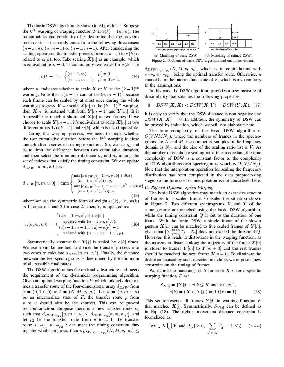
The basic DSW algorithm is shown in Algorithm 1.Suppose the kth warping of warping function F is c(k)=(n,m).The monotonicity and continuity of F determine that the previous -0 match c(k-1)can only come from the following three cases: a.33o333a a303033 (n-1,m),(n,m-1)or (n-1,m-1).After considering the mm+1m+2学m+3许m+4m+s mm+1m2外m43 scaling operation,the transfer process from c(k-1)to c()is (a)Matching of basic DSW. (b)Matching of refined DSW. related to a(k),too.Take scaling X[n]as an example,which Figure 2.Problem of basic DSW algorithm and our improvement is equivalent to u=0.There are only two cases for c(k-1): ck-1)=-1,m) dosw(N,M,),which is in contradiction with 4=0 (14) sp up2t being the optimal transfer route.Otherwise,u (n-1,m-1)4=0or1. cannot be in the intermediate state of F,which is also contrary to the assumptions. where u indicates whether to scale X or Y at the (k-1)th In this way,the DSW algorithm provides a new measure of warping.Note that c(k-1)cannot be (n,m -1),because dissimilarity that satisfies the following properties: each frame can be scaled by at most once during the whole warping progress.If we scale Xn]at the (k-1)th warping. 0=DSW(X,X)<DSW(X,Y)=DSW(Y,X).(17) then XIn]is matched with both Y[m-1]and Y[m].It is impossible to match a shortened Xn]to two frames.If we It is easy to verify that the DSW distance is non-negative and choose to scale Y[m-1],it's equivalent to scale X[n]at two DSW(X,X)=0.In addition,the symmetry of DSW can different ratios 1/ak-1]and a,which is also impossible. be proved by induction,which we will not elaborate here. During the warping process,we need to track whether The time complexity of the basic DSW algorithm is the two cumulative duration before the kth warping is close O(VNMN),where the numbers of frames in the spectro- enough after a series of scaling operations.So,we use gi and grams are N and M,the number of samples in the frequency g2 to limit the difference between two cumulative duration, domain is Nf,and the size of the scaling ratio list is V.As the number of candidate scaling ratio V is a constant,the time and then select the minimum distance di and d2 among the set of indexes that satisfy the timing constraint.We can update complexity of DSW is a constant factor to the complexity dpsw [n,m,v,0]as: of DTW algorithms over spectrograms,which is O(NMN). Note that the interpolation operation for scaling the frequency min{dpsw [n-1,m,v,0+dist distribution has been completed in the data preprocessing dpsw[n,m,v,0 min (n-1,m,v,0)∈q1 stage,so the time cost of interpolation is not considered here. min{dpswin-1,m-1,,]+2dist C.Refined Dynamic Speed Warping (n-1,m,v,u）Eq2 (15) The basic DSW algorithm may match an excessive amount where we use the symmetric form of weight w(k),i.e.,w(k) of frames to a scaled frame.Consider the situation shown is 1 for case 1 and 2 for case 2.Then,ls is updated as: in Figure 2.Two different spectrograms X and Y of the same gesture are matched using the basic DSW algorithm, (l.[n-1,m,v,O]+alv while the timing constraint O is set to the duration of one updated with (n-1,m,v,0); frame.With the basic DSW,a single frame of the slower ls[n,m,v,O]= (16) lsn-1,m-1,v,川+av]-1 gesture X[n]can be matched to five scaled frames of Y[n], updated with (n-1,m-1,v,u). given thatT does not exceed the threshold 1=m However,this leads to distortions in the warping function,as Symmetrically,assume that Yj]is scaled by a[k]times. the movement distance along the trajectory of the frame X[n] We use a similar method to divide the transfer process into is closer to frames Ym]to Y[m +3]and the rest frames two cases to calculate dpsw [n,m,v,1].Finally,the distance should be matched the next frame Xn+1].To eliminate the between the two spectrograms is determined by the minimum distortion caused by such repeated matching,we impose a new of all possible final states. constraint on the timing of frames. The DSW algorithm has the optimal substructure and meets We define the matching set S for each Xi]for a specific the requirement of the dynamical programming algorithm. warping function F as: Given an optimal warping function F,which uniquely determ- ines a transfer route of the four-dimensional array dpsw from Sx={Y[jl|3k≤K and k∈N+ s =(0,0,0,0)to t=(N,M,vt,ut).Let u (n,m,v,L) c(k)=(X[i],Yj])and I(k)=1) (18) be an intermediate state of F,the transfer route p from s to u should also be the shortest.This can be proved This set represents all frames Yj]in warping function F by contradiction.Suppose there is a new transfer route p that matched X[i.Symmetrically,Sylil can be defined as such that dpswn,m,v,udpswIn,m,v,ul,and in Eq.(18).The tighter movement distance constraint is let p2 be the transfer route from u to t.If the transfer formalized as: route spup2t can meet the timing constraint dur- z∈KUY and |S.l≥0，∑T:-1≤5.(*利 ing the whole progress,then dpsw(N,M,v)The basic DSW algorithm is shown in Algorithm 1. Suppose the kth warping of warping function F is c(k)=(n, m). The monotonicity and continuity of F determine that the previous match c (k￾1) can only come from the following three cases: (n￾1, m), (n, m￾1) or (n￾1, m￾1). After considering the scaling operation, the transfer process from c (k￾1) to c (k) is related to ↵(k), too. Take scaling X[n] as an example, which is equivalent to µ = 0. There are only two cases for c (k ￾1): c (k ￾ 1) = ⇢ (n ￾ 1, m) µ 0 = 0 (n ￾ 1, m ￾ 1) µ 0 = 0 or 1. (14) where µ 0 indicates whether to scale X or Y at the (k ￾ 1)th warping. Note that c (k ￾ 1) cannot be (n, m ￾ 1), because each frame can be scaled by at most once during the whole warping progress. If we scale X[n] at the (k ￾ 1)th warping, then X[n] is matched with both Y [m ￾ 1] and Y [m]. It is impossible to match a shortened X[n] to two frames. If we choose to scale Y [m￾1], it’s equivalent to scale X[n] at two different ratios 1/↵[k ￾ 1] and ↵[k], which is also impossible. During the warping process, we need to track whether the two cumulative duration before the kth warping is close enough after a series of scaling operations. So, we use q1 and q2 to limit the difference between two cumulative duration, and then select the minimum distance d1 and d2 among the set of indexes that satisfy the timing constraint. We can update dDSW [n, m, v, 0] as: dDSW [n, m, v, 0] = min 8 >< >: min{dDSW [n ￾ 1, m, v0 , 0] + dist} (n ￾ 1, m, v0 , 0) 2 q1 min{dDSW [n ￾ 1, m ￾ 1, v0 , µ0 ]+2 dist} (n ￾ 1, m, v0 , µ0 ) 2 q2 (15) where we use the symmetric form of weight w(k), i.e., w(k) is 1 for case 1 and 2 for case 2. Then, ls is updated as: ls[n, m, v, 0] = 8 >>< >>: ls[n ￾ 1, m, v0 , 0] + ↵[v 0 ] updated with (n ￾ 1, m, v0 , 0); ls[n ￾ 1, m ￾ 1, v0 , µ] + ↵[v 0 ] ￾ 1 updated with (n ￾ 1, m ￾ 1, v0 , µ). (16) Symmetrically, assume that Y [j] is scaled by ↵[k] times. We use a similar method to divide the transfer process into two cases to calculate dDSW [n, m, v, 1]. Finally, the distance between the two spectrograms is determined by the minimum of all possible final states. The DSW algorithm has the optimal substructure and meets the requirement of the dynamical programming algorithm. Given an optimal warping function F, which uniquely determ￾ines a transfer route of the four-dimensional array dDSW from s = (0, 0, 0, 0) to t = (N,M,vt, µt). Let u = (n, m, v, µ) be an intermediate state of F, the transfer route p from s to u should also be the shortest. This can be proved by contradiction. Suppose there is a new transfer route p1 such that dDSW;p1 [n, m, v, µ]  dDSW;p [n, m, v, µ], and let p2 be the transfer route from u to t. If the transfer route s ;p1 u ;p2 t can meet the timing constraint dur￾ing the whole progress, then dDSW;p1;p2 (N,M,vt, µt)  1 0.3 0.3 0.3 0.3 X Y nth mth (m+2)th (m+1)th 0.3 0.3 Q = 1 (m+3)th (m+4)th (m+5)th (a) Matching of basic DSW. 1 0.3 0.3 0.3 0.3 X Y nth mth (m+2)th (m+1)th ξ = 0.2 (m+3)th (b) Matching of refined DSW. Figure 2. Problem of basic DSW algorithm and our improvement. dDSW;p;p2 (N,M,vt, µt), which is in contradiction with s ;p u ;p2 t being the optimal transfer route. Otherwise, u cannot be in the intermediate state of F, which is also contrary to the assumptions. In this way, the DSW algorithm provides a new measure of dissimilarity that satisfies the following properties: 0 = DSW(X, X) < DSW(X,Y ) = DSW(Y , X). (17) It is easy to verify that the DSW distance is non-negative and DSW(X, X)=0. In addition, the symmetry of DSW can be proved by induction, which we will not elaborate here. The time complexity of the basic DSW algorithm is O(VNMNf ), where the numbers of frames in the spectro￾grams are N and M, the number of samples in the frequency domain is Nf , and the size of the scaling ratio list is V . As the number of candidate scaling ratio V is a constant, the time complexity of DSW is a constant factor to the complexity of DTW algorithms over spectrograms, which is O(NMNf ). Note that the interpolation operation for scaling the frequency distribution has been completed in the data preprocessing stage, so the time cost of interpolation is not considered here. C. Refined Dynamic Speed Warping The basic DSW algorithm may match an excessive amount of frames to a scaled frame. Consider the situation shown in Figure 2. Two different spectrograms X and Y of the same gesture are matched using the basic DSW algorithm, while the timing constraint Q is set to the duration of one frame. With the basic DSW, a single frame of the slower gesture X[n] can be matched to five scaled frames of Y [n], given that | Pm+5 j=m Tj ￾ Tn| does not exceed the threshold Q. However, this leads to distortions in the warping function, as the movement distance along the trajectory of the frame X[n] is closer to frames Y [m] to Y [m + 3] and the rest frames should be matched the next frame X[n + 1]. To eliminate the distortion caused by such repeated matching, we impose a new constraint on the timing of frames. We define the matching set S for each X[i] for a specific warping function F as: SX[i] = {Y [j] | 9 k  K and k 2 N +, c(k)=(X[i],Y [j]) and I(k)=1} (18) This set represents all frames Y [j] in warping function F that matched X[i]. Symmetrically, SY [j] can be defined as in Eq. (18). The tighter movement distance constraint is formalized as: 8z 2 X [Y and |Sz| ￾ 0, X z0 2Sz Tz0 ￾ 1  ⇠. (⇤⇤⇤)