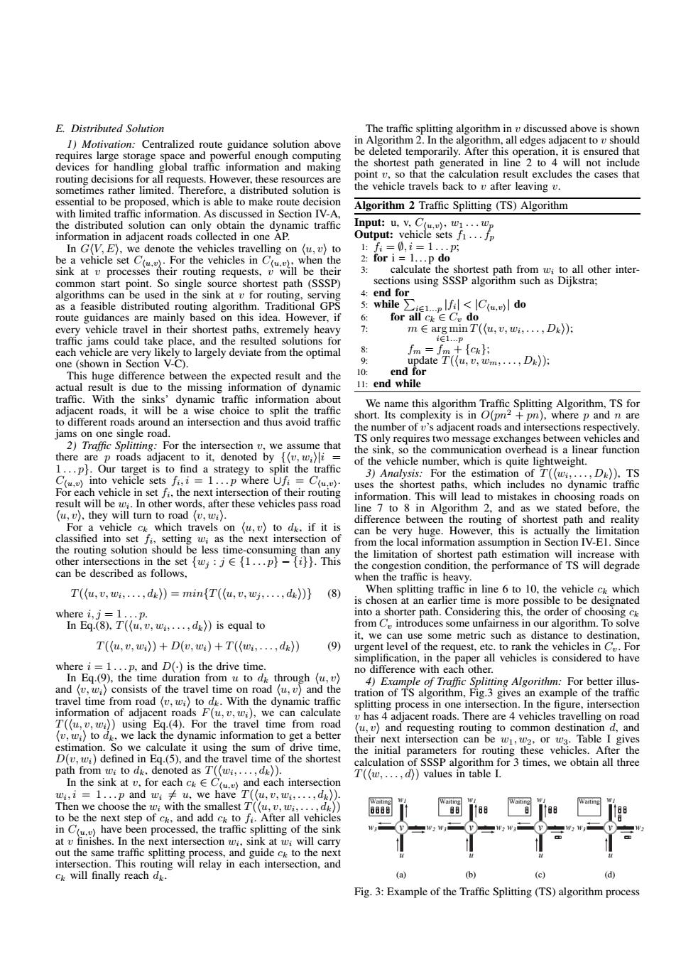
E.Distributed Solution The traffic splitting algorithm in v discussed above is shown 1)Motivation:Centralized route guidance solution above in Algorithm 2.In the algorithm,all edges adjacent to v should requires large storage space and powerful enough computing be deleted temporarily.After this operation.it is ensured that devices for handling global traffic information and making the shortest path generated in line 2 to 4 will not include routing decisions for all requests.However,these resources are point v.so that the calculation result excludes the cases that sometimes rather limited.Therefore.a distributed solution is the vehicle travels back to v after leaving v. essential to be proposed,which is able to make route decision Algorithm 2 Traffic Splitting (TS)Algorithm with limited traffic information.As discussed in Section IV-A the distributed solution can only obtain the dynamic traffic Input:u,v.Cuv),w1...wp information in adjacent roads collected in one AP. Output:vehicle sets f1...fp In G(V,E),we denote the vehicles travelling on (u,v)to 1:f=0,i=1..p be a vehicle set Cu)For the vehicles in Cu.)when the 2:for i 1...p do sink at v processes their routing requests,v will be their 3: calculate the shortest path from w;to all other inter- common start point.So single source shortest path (SSSP) sections using SSSP algorithm such as Dijkstra; algorithms can be used in the sink at v for routing,serving 4:end for as a feasible distributed routing algorithm.Traditional GPS 5:while ie..fil<C(u.v)l do route guidances are mainly based on this idea.However,if 6 for all ck∈Cudo every vehicle travel in their shortest paths,extremely heavy m∈arg min T(u,v,,,Dk)月 traffic jams could take place,and the resulted solutions for 1∈1..D each vehicle are very likely to largely deviate from the optimal 8: fm=fm+ick}; one (shown in Section V-C). 9: update T((u,v,wm,...,D)); This huge difference between the expected result and the 10 end for actual result is due to the missing information of dynamic 11:end while traffic.With the sinks'dynamic traffic information about We name this algorithm Traffic Splitting Algorithm,TS for adjacent roads,it will be a wise choice to split the traffic short.Its complexity is in O(pn-+pn),where p and n are to different roads around an intersection and thus avoid traffic the number of v's adjacent roads and intersections respectively. jams on one single road TS only requires two message exchanges between vehicles and 2)Traffic Splitting:For the intersection v,we assume that the sink,so the communication overhead is a linear function there are p roads adjacent to it,denoted by (v,w;i= 1...p}.Our target is to find a strategy to split the traffic of the vehicle number,which is quite lightweight. 3)Analysis:For the estimation of T((wi.....D)).TS Cu.v)into vehicle sets fi,i=1...p where Ufi =C(u.v). uses the shortest paths,which includes no dynamic traffic For each vehicle in set fi,the next intersection of their routing information.This will lead to mistakes in choosing roads on result will be w.In other words,after these vehicles pass road line 7 to 8 in Algorithm 2.and as we stated before,the (u,v),they will turn to road (v,wi). difference between the routing of shortest path and reality For a vehicle ck which travels on (u,v)to dk,if it is can be very huge.However,this is actually the limitation classified into set fi,setting wi as the next intersection of from the local information assumption in Section IV-E1.Since the routing solution should be less time-consuming than any the limitation of shortest path estimation will increase with other intersections in the set w;:jef1...p.This the congestion condition,the performance of TS will degrade can be described as follows, when the traffic is heavy. T((u,v,wi;...,dx))=minfT((u,v,wj;...,dx))} (8) When splitting traffic in line 6 to 10,the vehicle ck which is chosen at an earlier time is more possible to be designated where i,j=1...p. into a shorter path.Considering this,the order of choosing ck In Eq.(8),T((u,v.wi.....d)is equal to from C.,introduces some unfairness in our algorithm.To solve it,we can use some metric such as distance to destination T(u,U,)+D(v,w)+T(,,d) (9) urgent level of the request,etc.to rank the vehicles in Cv.For simplification,in the paper all vehicles is considered to have where i=1...p,and D()is the drive time. no difference with each other. In Eq.(9),the time duration from u to d through (u,v) 4)Example of Traffic Splitting Algorithm:For better illus- and (v,w;)consists of the travel time on road (u,v)and the tration of TS algorithm,Fig.3 gives an example of the traffic travel time from road (v.wi)to dk.With the dynamic traffic information of adjacent roads F(u,v,wi),we can calculate splitting process in one intersection.In the figure,intersection v has 4 adjacent roads.There are 4 vehicles travelling on road T((u,v,wi))using Eq.(4).For the travel time from road u,v)and requesting routing to common destination d,and (v,w)to dk,we lack the dynamic information to get a better their next intersection can be w1,w2,or w3.Table I gives estimation.So we calculate it using the sum of drive time. the initial parameters for routing these vehicles.After the D(v,wi)defined in Eq.(5),and the travel time of the shortest calculation of SSSP algorithm for 3 times,we obtain all three path from wi to dk,denoted as T(wi,...,d)). T((w,...,d))values in table I. In the sink at v,for each ckECu and each intersection ,i=1.…p and w:≠u,we have T(u,v,u,,dk) Then we choose the wi with the smallest T((u,v,wi,...,d)) to be the next step of ck,and add ck to fi.After all vehicles in C)have been processed,the traffic splitting of the sink at v finishes.In the next intersection wi.sink at w;will carry out the same traffic splitting process,and guide ck to the next intersection.This routing will relay in each intersection,and ck will finally reach dk. (c) (d) Fig.3:Example of the Traffic Splitting (TS)algorithm processE. Distributed Solution 1) Motivation: Centralized route guidance solution above requires large storage space and powerful enough computing devices for handling global traffic information and making routing decisions for all requests. However, these resources are sometimes rather limited. Therefore, a distributed solution is essential to be proposed, which is able to make route decision with limited traffic information. As discussed in Section IV-A, the distributed solution can only obtain the dynamic traffic information in adjacent roads collected in one AP. In GhV, Ei, we denote the vehicles travelling on hu, vi to be a vehicle set Chu,vi . For the vehicles in Chu,vi , when the sink at v processes their routing requests, v will be their common start point. So single source shortest path (SSSP) algorithms can be used in the sink at v for routing, serving as a feasible distributed routing algorithm. Traditional GPS route guidances are mainly based on this idea. However, if every vehicle travel in their shortest paths, extremely heavy traffic jams could take place, and the resulted solutions for each vehicle are very likely to largely deviate from the optimal one (shown in Section V-C). This huge difference between the expected result and the actual result is due to the missing information of dynamic traffic. With the sinks’ dynamic traffic information about adjacent roads, it will be a wise choice to split the traffic to different roads around an intersection and thus avoid traffic jams on one single road. 2) Traffic Splitting: For the intersection v, we assume that there are p roads adjacent to it, denoted by {hv, wii|i = 1 . . . p}. Our target is to find a strategy to split the traffic Chu,vi into vehicle sets fi , i = 1 . . . p where ∪fi = Chu,vi . For each vehicle in set fi , the next intersection of their routing result will be wi . In other words, after these vehicles pass road hu, vi, they will turn to road hv, wii. For a vehicle ck which travels on hu, vi to dk, if it is classified into set fi , setting wi as the next intersection of the routing solution should be less time-consuming than any other intersections in the set {wj : j ∈ {1 . . . p} − {i}}. This can be described as follows, T (hu, v, wi , . . . , dki) = min{T (hu, v, wj, . . . , dki)} (8) where i, j = 1 . . . p. In Eq.(8), T (hu, v, wi , . . . , dki) is equal to T (hu, v, wii) + D(v, wi) + T (hwi , . . . , dki) (9) where i = 1 . . . p, and D(·) is the drive time. In Eq.(9), the time duration from u to dk through hu, vi and hv, wii consists of the travel time on road hu, vi and the travel time from road hv, wii to dk. With the dynamic traffic information of adjacent roads F(u, v, wi), we can calculate T (hu, v, wii) using Eq.(4). For the travel time from road hv, wii to dk, we lack the dynamic information to get a better estimation. So we calculate it using the sum of drive time, D(v, wi) defined in Eq.(5), and the travel time of the shortest path from wi to dk, denoted as T (hwi , . . . , dki). In the sink at v, for each ck ∈ Chu,vi and each intersection wi , i = 1 . . . p and wi 6= u, we have T (hu, v, wi , . . . , dki). Then we choose the wi with the smallest T (hu, v, wi , . . . , dki) to be the next step of ck, and add ck to fi . After all vehicles in Chu,vi have been processed, the traffic splitting of the sink at v finishes. In the next intersection wi , sink at wi will carry out the same traffic splitting process, and guide ck to the next intersection. This routing will relay in each intersection, and ck will finally reach dk. The traffic splitting algorithm in v discussed above is shown in Algorithm 2. In the algorithm, all edges adjacent to v should be deleted temporarily. After this operation, it is ensured that the shortest path generated in line 2 to 4 will not include point v, so that the calculation result excludes the cases that the vehicle travels back to v after leaving v. Algorithm 2 Traffic Splitting (TS) Algorithm Input: u, v, Chu,vi , w1 . . . wp Output: vehicle sets f1 . . . fp 1: fi = ∅, i = 1 . . . p; 2: for i = 1. . . p do 3: calculate the shortest path from wi to all other inter￾sections using SSSP algorithm such as Dijkstra; 4: end for 5: while P i∈1...p |fi | < |Chu,vi | do 6: for all ck ∈ Cv do 7: m ∈ arg min i∈1...p T (hu, v, wi , . . . , Dki); 8: fm = fm + {ck}; 9: update T (hu, v, wm, . . . , Dki); 10: end for 11: end while We name this algorithm Traffic Splitting Algorithm, TS for short. Its complexity is in O(pn2 + pn), where p and n are the number of v’s adjacent roads and intersections respectively. TS only requires two message exchanges between vehicles and the sink, so the communication overhead is a linear function of the vehicle number, which is quite lightweight. 3) Analysis: For the estimation of T (hwi , . . . , Dki), TS uses the shortest paths, which includes no dynamic traffic information. This will lead to mistakes in choosing roads on line 7 to 8 in Algorithm 2, and as we stated before, the difference between the routing of shortest path and reality can be very huge. However, this is actually the limitation from the local information assumption in Section IV-E1. Since the limitation of shortest path estimation will increase with the congestion condition, the performance of TS will degrade when the traffic is heavy. When splitting traffic in line 6 to 10, the vehicle ck which is chosen at an earlier time is more possible to be designated into a shorter path. Considering this, the order of choosing ck from Cv introduces some unfairness in our algorithm. To solve it, we can use some metric such as distance to destination, urgent level of the request, etc. to rank the vehicles in Cv. For simplification, in the paper all vehicles is considered to have no difference with each other. 4) Example of Traffic Splitting Algorithm: For better illus￾tration of TS algorithm, Fig.3 gives an example of the traffic splitting process in one intersection. In the figure, intersection v has 4 adjacent roads. There are 4 vehicles travelling on road hu, vi and requesting routing to common destination d, and their next intersection can be w1, w2, or w3. Table I gives the initial parameters for routing these vehicles. After the calculation of SSSP algorithm for 3 times, we obtain all three T (hw, . . . , di) values in table I. v 9 w1 w3 w2 Waiting u (a) v 9 w1 w3 w2 Waiting u (b) v 9 w1 w3 w2 Waiting u (c) v 9 w1 w3 w2 Waiting u (d) Fig. 3: Example of the Traffic Splitting (TS) algorithm process