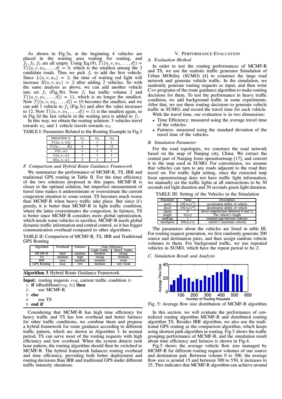
As shown in Fig.3a,at the beginning 4 vehicles are V.PERFORMANCE EVALUATION placed in the waiting area waiting for routing,and A.Evaluation Method fi f2,f3 are all empty.Using Eq.(9).T((u,v,w1,....d))= T((u,v,w2,...,d)=9,which is the smallest among the 3 In order to test the routing performances of MCMF-R candidate roads.Thus we pick f to add the first vehicle. and TS,we use the realistic traffic generator Simulation of Since L(u,v,w1)=2,the time of waiting red light will Urban MObility (SUMO)[4]to construct the large road increase R(u,v.w1)=2 after adding 2 vehicles.So with network and generate vehicle traffic.In the simulation,we the same analysis as above,we can add another vehicle randomly generate routing requests as input,and then write into set f (Fig.3b).Now fi has traffic volume 2 and C++programs of the route guidance algorithm to make routing T((u,v,w1,...,d))=11,which is no longer the smallest. decisions for them.To test the performance in heavy traffic Now T((u,v,w2,...,d))=10 becomes the smallest,and we condition,we add background traffic in some experiments. can add 1 vehicle to f2(Fig.3c)and after the value increases After that,we use these routing decisions to generate vehicle to 12.Now T(u,v,w1: ...d))=11 is the smallest again,so traffic in SUMO,and record the travel time for each vehicle. in Fig.3d the last vehicle in the waiting area is added to f1. With the travel time,our evaluation is in two dimensions: In this way,we obtain the routing solution:3 vehicles travel Time Efficiency:measured using the average travel time towards w and 1 vehicle travels towards w2. of the vehicles. TABLE I:Parameters Related to the Routing Example in Fig.3 Fairness:measured using the standard deviation of the travel time of the vehicles. intersection w T(u,,四) B.Simulation Parameter 1《0、....d】 6 2 For the road topologies,we construct the road network LD（U.心) L(u,, based on the map of Nanjing city,China.We extract the L.U.D】 central part of Nanjing from openstreetmap [17],and convert it to the map used in SUMO.For convenience,we assume F.Comparison and Hybrid Route Guidance framework that vehicles can turn to any roads adjacent to the road they We summarize the performance of MCMF-R,TS,IRR and travel on.For traffic light setting,since the extracted map traditional GPS routing in Table II.For the time efficiency from openstreetmap does not have traffic light information of the two solutions proposed in this paper,MCMF-R is we manually set the traffic lights at all intersections to be 30 closer to the optimal solution,but imperfect measurement of seconds red light duration and 30 seconds green light duration. travel time makes it underestimate or overestimate the current congestion situation to some extent.TS becomes much worse TABLE III:Setting of the Vehicles in the Simulation than MCMF-R when heavy traffic take place.But since it's Parameter Value ●escnption greedy,it is better than MCMF-R in light traffic condition, accel 10(m/s) acceleration ability of vehicle decel 10(m/s2) deceleration ability of vehicle where the latter overestimates the congestion.In fairness.TS sigma driver imperfection (between 0 and I) is better since MCMF-R considers more global optimization, 3m】 The vehicle's length which needs some vehicles to sacrifice.MCMF-R needs global nimal gap bet en maxSpeed 80(m/s) vehicle's maximum velocity dynamic traffic information and central control,so it has bigger communication overhead compared to other algorithms. The parameters about the vehicles are listed in table III TABLE II:Comparison of MCMF-R,TS,IRR and Traditional For routing request generation,we first randomly generate 200 GPS Routing source and destination pairs,and then assign random vehicle volumes to them.For background traffic,we use repeated Algorithm Overhead Light Tn vehicles in SUMO,which have the repeat period to be 2. MCME-R C.Simulation Result and Analysis GPS Routing casv ow medium very weak 840 Algorithm 3 Hybrid Route Guidance Framework Input:routing requests reg,current traffic condition tc 1:if isRushHour(req,tc)then use MCMF-R 3:else 100 200300 400500 600 use TS Number of Routing Requests 5:end if Fig.5:Average flow size distribution of MCMF-R algorithm Considering that MCMF-R has high time efficiency for In this section.we will evaluate the performance of cen- heavy traffic and TS has low overhead and better fairness tralized routing algorithm MCMF-R and distributed routing for other traffic conditions,we combine them and propose algorithm TS.Besides IRR algorithm,we also use the tradi- a hybrid framework for route guidance according to different tional GPS routing as the comparison algorithm,which keeps traffic pattern,which are shown in Algorithm 3.In normal using shortest path algorithm in routing.Fig.5 shows the traffic period,TS can serve most of the routing requests with high grouping performance of MCMF-R,and the simulation result efficiency and low overhead.When the system detects rush about time efficiency and fairness is shown in Fig.4. hour pattern,the routing algorithm should then be switched to Fig.5 shows the average vehicle flow size managed by MCMF-R.The hybrid framework balances routing overhead MCMF-R for different routing request volumes of one source and time efficiency,providing both better deployment and and destination pair.Between volume 0 to 300,the average routing decisions than IRR and traditional GPS under different flow size is around 15 and between 300 to 550,it increases to traffic intensity situations. 25.This indicates that MCMF-R algorithm can achieve aroundAs shown in Fig.3a, at the beginning 4 vehicles are placed in the waiting area waiting for routing, and f1, f2, f3 are all empty. Using Eq.(9), T (hu, v, w1, . . . , di) = T (hu, v, w2, . . . , di = 9, which is the smallest among the 3 candidate roads. Thus we pick f1 to add the first vehicle. Since L(u, v, w1) = 2, the time of waiting red light will increase R(u, v, w1) = 2 after adding 2 vehicles. So with the same analysis as above, we can add another vehicle into set f1 (Fig.3b). Now f1 has traffic volume 2 and T (hu, v, w1, . . . , di) = 11, which is no longer the smallest. Now T (hu, v, w2, . . . , di) = 10 becomes the smallest, and we can add 1 vehicle to f2 (Fig.3c) and after the value increases to 12. Now T (hu, v, w1, . . . , di) = 11 is the smallest again, so in Fig.3d the last vehicle in the waiting area is added to f1. In this way, we obtain the routing solution: 3 vehicles travel towards w1 and 1 vehicle travels towards w2. TABLE I: Parameters Related to the Routing Example in Fig.3 intersection w w1 w2 w3 T(hu, v, wi) 2 1 1 T(hw, . . . , di) 6 7 12 D(v, w) 1 2 1 L(u, v, w) 2 1 1 R(u, v, w) 2 2 1 F. Comparison and Hybrid Route Guidance Framework We summarize the performance of MCMF-R, TS, IRR and traditional GPS routing in Table II. For the time efficiency of the two solutions proposed in this paper, MCMF-R is closer to the optimal solution, but imperfect measurement of travel time makes it underestimate or overestimate the current congestion situation to some extent. TS becomes much worse than MCMF-R when heavy traffic take place. But since it’s greedy, it is better than MCMF-R in light traffic condition, where the latter overestimates the congestion. In fairness, TS is better since MCMF-R considers more global optimization, which needs some vehicles to sacrifice. MCMF-R needs global dynamic traffic information and central control, so it has bigger communication overhead compared to other algorithms. TABLE II: Comparison of MCMF-R, TS, IRR and Traditional GPS Routing Algorithm Overhead Fairness Time Efficiency Light Traffic Heavy Traffic MCMF-R hard medium medium strong TS medium high strong medium IRR easy medium medium weak GPS Routing easy low medium very weak Algorithm 3 Hybrid Route Guidance Framework Input: routing requests req, current traffic condition tc 1: if isRushHour(req, tc) then 2: use MCMF-R 3: else 4: use TS 5: end if Considering that MCMF-R has high time efficiency for heavy traffic and TS has low overhead and better fairness for other traffic conditions, we combine them and propose a hybrid framework for route guidance according to different traffic pattern, which are shown in Algorithm 3. In normal period, TS can serve most of the routing requests with high efficiency and low overhead. When the system detects rush hour pattern, the routing algorithm should then be switched to MCMF-R. The hybrid framework balances routing overhead and time efficiency, providing both better deployment and routing decisions than IRR and traditional GPS under different traffic intensity situations. V. PERFORMANCE EVALUATION A. Evaluation Method In order to test the routing performances of MCMF-R and TS, we use the realistic traffic generator Simulation of Urban MObility (SUMO) [4] to construct the large road network and generate vehicle traffic. In the simulation, we randomly generate routing requests as input, and then write C++ programs of the route guidance algorithm to make routing decisions for them. To test the performance in heavy traffic condition, we add background traffic in some experiments. After that, we use these routing decisions to generate vehicle traffic in SUMO, and record the travel time for each vehicle. With the travel time, our evaluation is in two dimensions: • Time Efficiency: measured using the average travel time of the vehicles. • Fairness: measured using the standard deviation of the travel time of the vehicles. B. Simulation Parameter For the road topologies, we construct the road network based on the map of Nanjing city, China. We extract the central part of Nanjing from openstreetmap [17], and convert it to the map used in SUMO. For convenience, we assume that vehicles can turn to any roads adjacent to the road they travel on. For traffic light setting, since the extracted map from openstreetmap does not have traffic light information, we manually set the traffic lights at all intersections to be 30 seconds red light duration and 30 seconds green light duration. TABLE III: Setting of the Vehicles in the Simulation Parameter Value Description accel 10(m/s2 ) acceleration ability of vehicle decel 10(m/s2 ) deceleration ability of vehicle sigma 0 driver imperfection (between 0 and 1) length 3(m) The vehicle’s length minGap 1 minimal gap between vehicles maxSpeed 80(m/s) vehicle’s maximum velocity The parameters about the vehicles are listed in table III. For routing request generation, we first randomly generate 200 source and destination pairs, and then assign random vehicle volumes to them. For background traffic, we use repeated vehicles in SUMO, which have the repeat period to be 2. C. Simulation Result and Analysis 100 200 300 400 500 600 0 20 40 Number of Routing Requests Average Flow Size Fig. 5: Average flow size distribution of MCMF-R algorithm In this section, we will evaluate the performance of cen￾tralized routing algorithm MCMF-R and distributed routing algorithm TS. Besides IRR algorithm, we also use the tradi￾tional GPS routing as the comparison algorithm, which keeps using shortest path algorithm in routing. Fig.5 shows the traffic grouping performance of MCMF-R, and the simulation result about time efficiency and fairness is shown in Fig.4. Fig.5 shows the average vehicle flow size managed by MCMF-R for different routing request volumes of one source and destination pair. Between volume 0 to 300, the average flow size is around 15 and between 300 to 550, it increases to 25. This indicates that MCMF-R algorithm can achieve around