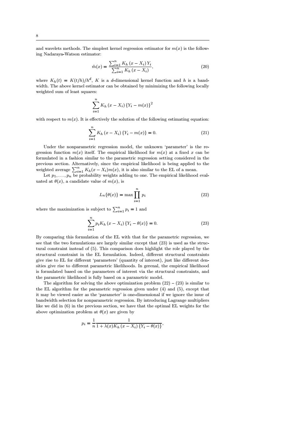
and wavelets methods.The simplest kernel regression estimator for m(r)is the follow- ing Nadaraya-Watson estimator: m(x）= ∑Kae-X)y (20) ∑=1Kh(e-X) where Kh(t)=K(t/h)/hd,K is a d-dimensional kernel function and h is a band- width.The above kernel estimator can be obtained by minimizing the following locally weighted sum of least squares: ∑Ke-X)出-m(}2 i= with respect to m(r).It is effectively the solution of the following estimating equation: Kae-X化-me=0 (21) i=1 Under the nonparametric regression model,the unknown 'parameter'is the re- gression function m(r)itself.The empirical likelihood for m()at a fixed x can be formulated in a fashion similar to the parametric regression setting considered in the previous section.Alternatively,since the empirical likelihood is being applied to the weighted average()m(),it is also similar to the EL of a mean. Let pi,...,Pn be probability weights adding to one.The empirical likelihood eval- uated at 0(x),a candidate value of m(r),is Ln{(e}=maxⅡn (22) 三1 where the maximization is subject toPi1and n p,Kh(e-X){Y-9}=0. (23) =1 By comparing this formulation of the EL with that for the parametric regression,we see that the two formulations are largely similar except that (23)is used as the struc- tural constraint instead of(5).This comparison does highlight the role played by the structural constraint in the EL formulation.Indeed,different structural constraints give rise to EL for different 'parameters'(quantity of interest),just like different den- sities give rise to different parametric likelihoods.In gerenal,the empirical likelihood is formulated based on the parameters of interest via the structural constraints,and the parametric likelihood is fully based on a parametric model. The algorithm for solving the above optimization problem(22)-(23)is similar to the EL algorithm for the parametric regression given under (4)and (5),except that it may be viewed easier as the parameter'is one-dimensional if we ignore the issue of bandwidth selection for nonparametric regression.By introducing Lagrange multipliers like we did in (6)in the previous section,we have that the optimal EL weights for the above optimization problem at 0(r)are given by 1。 Pi= n1+(x)Kh(-Xi){Yi-0()}8 and wavelets methods. The simplest kernel regression estimator for m(x) is the follow￾ing Nadaraya-Watson estimator: mˆ (x) = Pn P i=1 Kh (x − Xi) Yi n i=1 Kh (x − Xi) , (20) where Kh(t) = K(t/h)/hd , K is a d-dimensional kernel function and h is a band￾width. The above kernel estimator can be obtained by minimizing the following locally weighted sum of least squares: Xn i=1 Kh (x − Xi) {Yi − m(x)} 2 with respect to m(x). It is effectively the solution of the following estimating equation: Xn i=1 Kh (x − Xi) {Yi − m(x)} = 0. (21) Under the nonparametric regression model, the unknown ‘parameter’ is the re￾gression function m(x) itself. The empirical likelihood for m(x) at a fixed x can be formulated in a fashion similar to the parametric regression setting considered in the previous section. Alternatively, since the empirical likelihood is being applied to the weighted average Pn i=1 Kh(x − Xi)m(x), it is also similar to the EL of a mean. Let p1, . . . , pn be probability weights adding to one. The empirical likelihood eval￾uated at θ(x), a candidate value of m(x), is Ln{θ(x)} = maxYn i=1 pi (22) where the maximization is subject to Pn i=1 pi = 1 and Xn i=1 piKh (x − Xi) {Yi − θ(x)} = 0. (23) By comparing this formulation of the EL with that for the parametric regression, we see that the two formulations are largely similar except that (23) is used as the struc￾tural constraint instead of (5). This comparison does highlight the role played by the structural constraint in the EL formulation. Indeed, different structural constraints give rise to EL for different ‘parameters’ (quantity of interest), just like different den￾sities give rise to different parametric likelihoods. In gerenal, the empirical likelihood is formulated based on the parameters of interest via the structural constraints, and the parametric likelihood is fully based on a parametric model. The algorithm for solving the above optimization problem (22) – (23) is similar to the EL algorithm for the parametric regression given under (4) and (5), except that it may be viewed easier as the ‘parameter’ is one-dimensional if we ignore the issue of bandwidth selection for nonparametric regression. By introducing Lagrange multipliers like we did in (6) in the previous section, we have that the optimal EL weights for the above optimization problem at θ(x) are given by pi = 1 n 1 1 + λ(x)Kh (x − Xi) {Yi − θ(x)}