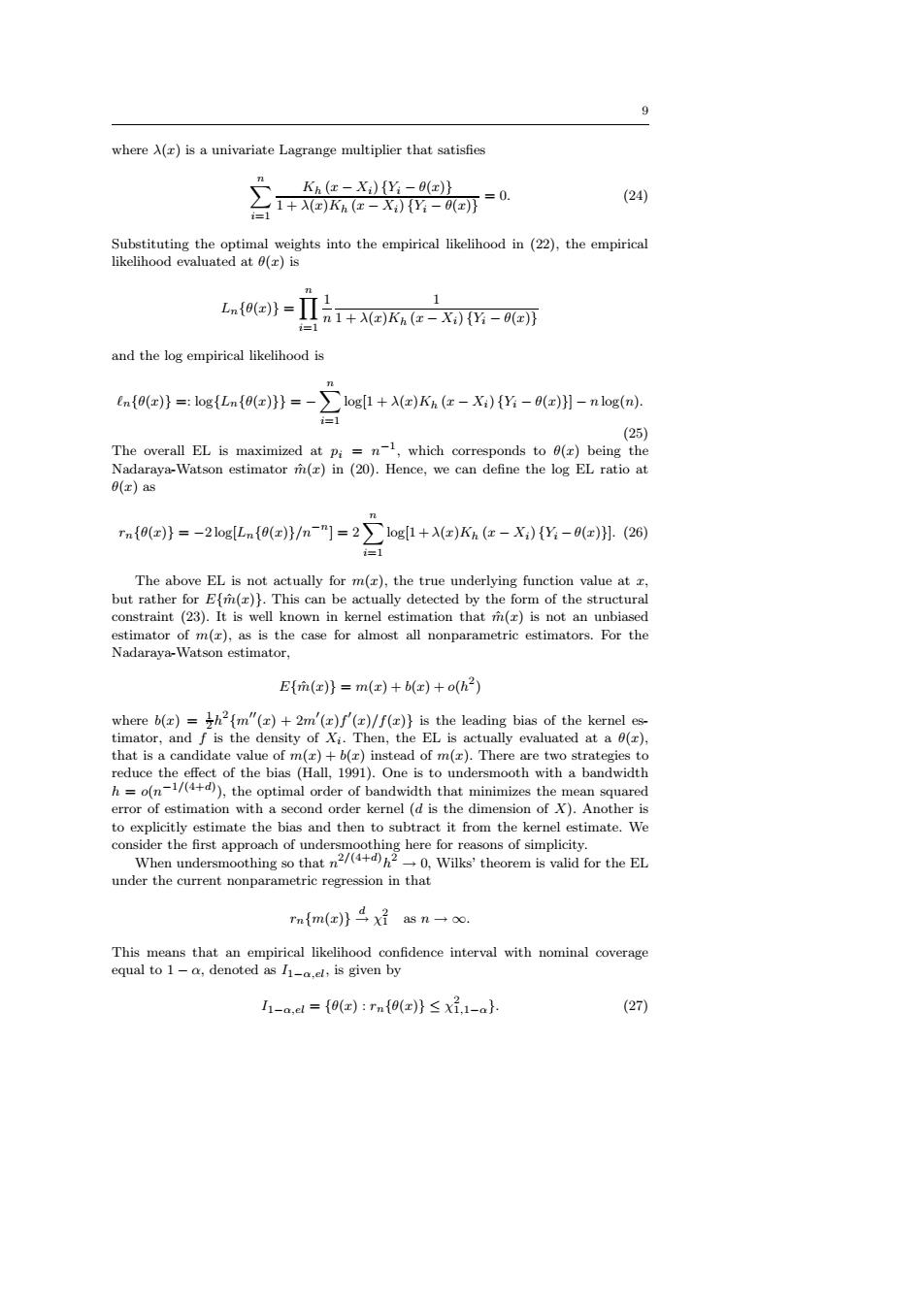
9 where A(x)is a univariate Lagrange multiplier that satisfies Kh(x-X){Y-0(x)} ∑1+A0-可=0 (24) Substituting the optimal weights into the empirical likelihood in(22),the empirical likelihood evaluated at 0(x)is Ln0}=Πh1+A四Ke-X)-oo i=1 and the log empirical likelihood is in{0(x)}=log{Ln{0(x)}}=->log1+X()Kn(-X:){Y:-0(x)}]-nlog(n). =1 (25) The overall EL is maximized at pi=n-1,which corresponds to 0(z)being the Nadaraya-Watson estimator m()in (20).Hence,we can define the log EL ratio at 0(x）as rn{0(x)}=-2log[Ln{0(x)}/m-n]=21og[1+A(x)Kh(x-X)Y-0(x)l.(26) =1 The above EL is not actually for m(x),the true underlying function value at z, but rather for Efm(z).This can be actually detected by the form of the structural constraint (23).It is well known in kernel estimation that m(x)is not an unbiased estimator of m(r),as is the case for almost all nonparametric estimators.For the Nadaraya-Watson estimator, E{m(x)}=m(x)+b(x)+o(h2) where b(r)=th2m"(r)+2m'(r)f'()/f(r)}is the leading bias of the kernel es- timator,and f is the density of Xi.Then,the EL is actually evaluated at a 0(), that is a candidate value of m()+b(r)instead of m(x).There are two strategies to reduce the effect of the bias (Hall,1991).One is to undersmooth with a bandwidth h=o(n/(4+),the optimal order of bandwidth that minimizes the mean squared error of estimation with a second order kernel (d is the dimension of X).Another is to explicitly estimate the bias and then to subtract it from the kernel estimate.We consider the first approach of undersmoothing here for reasons of simplicity. When undersmoothing so that n2/(+0,Wilks'theorem is valid for the EL under the current nonparametric regression in that rn{m(e}4X好asn→oo. This means that an empirical likelihood confidence interval with nominal coverage equal to 1-a,denoted as I1-a.el,is given by 11-a.el ={0()rnfo(r)}s xi.1-a}. (27)9 where λ(x) is a univariate Lagrange multiplier that satisfies Xn i=1 Kh (x − Xi) {Yi − θ(x)} 1 + λ(x)Kh (x − Xi) {Yi − θ(x)} = 0. (24) Substituting the optimal weights into the empirical likelihood in (22), the empirical likelihood evaluated at θ(x) is Ln{θ(x)} = Yn i=1 1 n 1 1 + λ(x)Kh (x − Xi) {Yi − θ(x)} and the log empirical likelihood is ℓn{θ(x)} =: log{Ln{θ(x)}} = − Xn i=1 log[1 + λ(x)Kh (x − Xi) {Yi − θ(x)}] − n log(n). (25) The overall EL is maximized at pi = n −1 , which corresponds to θ(x) being the Nadaraya-Watson estimator ˆm(x) in (20). Hence, we can define the log EL ratio at θ(x) as rn{θ(x)} = −2 log[Ln{θ(x)}/n−n ] = 2Xn i=1 log[1 + λ(x)Kh (x − Xi) {Yi − θ(x)}]. (26) The above EL is not actually for m(x), the true underlying function value at x, but rather for E{mˆ (x)}. This can be actually detected by the form of the structural constraint (23). It is well known in kernel estimation that ˆm(x) is not an unbiased estimator of m(x), as is the case for almost all nonparametric estimators. For the Nadaraya-Watson estimator, E{mˆ (x)} = m(x) + b(x) + o(h 2 ) where b(x) = 1 2 h 2 {m′′(x) + 2m′ (x)f ′ (x)/f(x)} is the leading bias of the kernel es￾timator, and f is the density of Xi . Then, the EL is actually evaluated at a θ(x), that is a candidate value of m(x) + b(x) instead of m(x). There are two strategies to reduce the effect of the bias (Hall, 1991). One is to undersmooth with a bandwidth h = o(n −1/(4+d) ), the optimal order of bandwidth that minimizes the mean squared error of estimation with a second order kernel (d is the dimension of X). Another is to explicitly estimate the bias and then to subtract it from the kernel estimate. We consider the first approach of undersmoothing here for reasons of simplicity. When undersmoothing so that n 2/(4+d)h 2 → 0, Wilks’ theorem is valid for the EL under the current nonparametric regression in that rn{m(x)} d→ χ 2 1 as n → ∞. This means that an empirical likelihood confidence interval with nominal coverage equal to 1 − α, denoted as I1−α,el, is given by I1−α,el = {θ(x) : rn{θ(x)} ≤ χ 2 1,1−α}. (27)