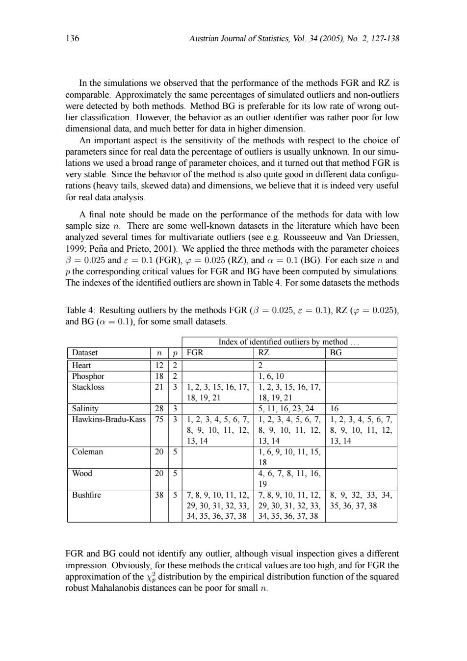
136 Austrian Journal of Statistics,Vol.34(2005),No.2,127-138 In the simulations we observed that the performance of the methods FGR and RZ is comparable.Approximately the same percentages of simulated outliers and non-outliers were detected by both methods.Method BG is preferable for its low rate of wrong out- lier classification.However,the behavior as an outlier identifier was rather poor for low dimensional data,and much better for data in higher dimension. An important aspect is the sensitivity of the methods with respect to the choice of parameters since for real data the percentage of outliers is usually unknown.In our simu- lations we used a broad range of parameter choices,and it turned out that method FGR is very stable.Since the behavior of the method is also quite good in different data configu- rations(heavy tails,skewed data)and dimensions,we believe that it is indeed very useful for real data analysis. A final note should be made on the performance of the methods for data with low sample size n.There are some well-known datasets in the literature which have been analyzed several times for multivariate outliers (see e.g.Rousseeuw and Van Driessen, 1999;Pena and Prieto,2001).We applied the three methods with the parameter choices B=0.025 and e=0.1 (FGR),=0.025(RZ),and a 0.1 (BG).For each size n and p the corresponding critical values for FGR and BG have been computed by simulations. The indexes of the identified outliers are shown in Table 4.For some datasets the methods Table 4:Resulting outliers by the methods FGR(B=0.025,=0.1),RZ (=0.025), and BG (a =0.1),for some small datasets. Index of identified outliers by method... Dataset n P FGR RZ BG Heart 122 2 Phosphor 18 2 1,6.10 Stackloss 21 1,2,3,15,16,17, 1,2,3,15,16,17 18,19,21 1819,21 Salinity 283 5,11,16,23,24 16 Hawkins-Bradu-Kass 75 3 1,2,3,4,5,6,7, 1,2,3,4,5,6,7,1,2,3,4,5,6,7 8,9,10,11,12, 8,9,10,11,12, 8,9,10,11,12, 13,14 13,14 13,14 Coleman 205 1,69,10,11,15, 18 Wood 20 5 4,6,7,8,11,16 19 Bushfire 38 5 7,8,9,10,11,12, 7,8,9,10,11,12,8,9,32,33,34, 29,30,31,32,33, 29,30,31,32,33 35,36,37,38 34,35,36,37,38 34,35,36,37,38 FGR and BG could not identify any outlier,although visual inspection gives a different impression.Obviously,for these methods the critical values are too high,and for FGR the approximation of the x2 distribution by the empirical distribution function of the squared robust Mahalanobis distances can be poor for small n.136 Austrian Journal of Statistics, Vol. 34 (2005), No. 2, 127-138 In the simulations we observed that the performance of the methods FGR and RZ is comparable. Approximately the same percentages of simulated outliers and non-outliers were detected by both methods. Method BG is preferable for its low rate of wrong out￾lier classification. However, the behavior as an outlier identifier was rather poor for low dimensional data, and much better for data in higher dimension. An important aspect is the sensitivity of the methods with respect to the choice of parameters since for real data the percentage of outliers is usually unknown. In our simu￾lations we used a broad range of parameter choices, and it turned out that method FGR is very stable. Since the behavior of the method is also quite good in different data configu￾rations (heavy tails, skewed data) and dimensions, we believe that it is indeed very useful for real data analysis. A final note should be made on the performance of the methods for data with low sample size n. There are some well-known datasets in the literature which have been analyzed several times for multivariate outliers (see e.g. Rousseeuw and Van Driessen, 1999; Pena and Prieto, 2001). We applied the three methods with the parameter choices ˜ β = 0.025 and ε = 0.1 (FGR), ϕ = 0.025 (RZ), and α = 0.1 (BG). For each size n and p the corresponding critical values for FGR and BG have been computed by simulations. The indexes of the identified outliers are shown in Table 4. For some datasets the methods Table 4: Resulting outliers by the methods FGR (β = 0.025, ε = 0.1), RZ (ϕ = 0.025), and BG (α = 0.1), for some small datasets. Index of identified outliers by method . . . Dataset n p FGR RZ BG Heart 12 2 2 Phosphor 18 2 1, 6, 10 Stackloss 21 3 1, 2, 3, 15, 16, 17, 18, 19, 21 1, 2, 3, 15, 16, 17, 18, 19, 21 Salinity 28 3 5, 11, 16, 23, 24 16 Hawkins-Bradu-Kass 75 3 1, 2, 3, 4, 5, 6, 7, 8, 9, 10, 11, 12, 13, 14 1, 2, 3, 4, 5, 6, 7, 8, 9, 10, 11, 12, 13, 14 1, 2, 3, 4, 5, 6, 7, 8, 9, 10, 11, 12, 13, 14 Coleman 20 5 1, 6, 9, 10, 11, 15, 18 Wood 20 5 4, 6, 7, 8, 11, 16, 19 Bushfire 38 5 7, 8, 9, 10, 11, 12, 29, 30, 31, 32, 33, 34, 35, 36, 37, 38 7, 8, 9, 10, 11, 12, 29, 30, 31, 32, 33, 34, 35, 36, 37, 38 8, 9, 32, 33, 34, 35, 36, 37, 38 FGR and BG could not identify any outlier, although visual inspection gives a different impression. Obviously, for these methods the critical values are too high, and for FGR the approximation of the χ 2 p distribution by the empirical distribution function of the squared robust Mahalanobis distances can be poor for small n