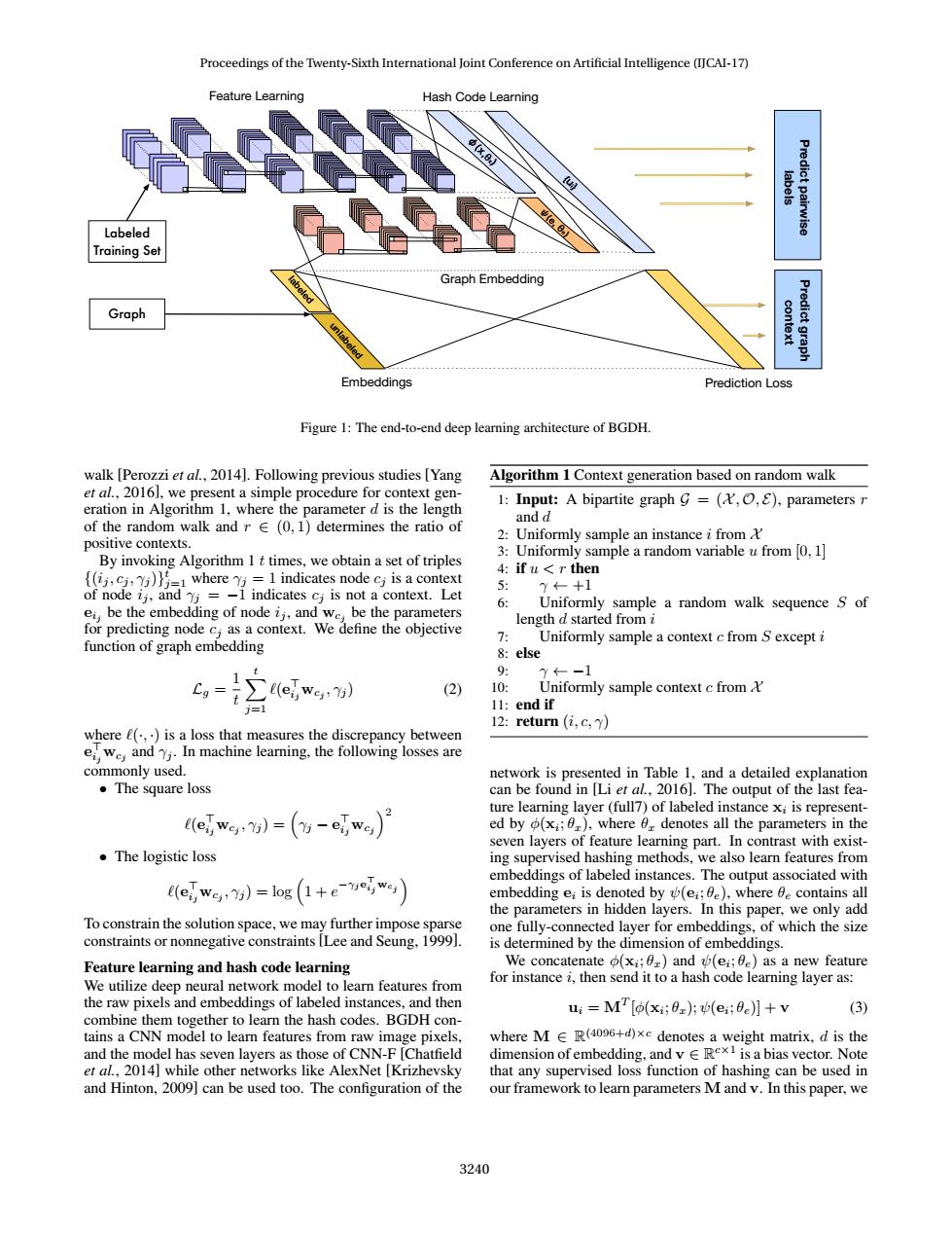
Proceedings of the Twenty-Sixth International Joint Conference on Artificial Intelligence (IJCAI-17) Feature Learning Hash Code Learning labels Predict pairwise Labeled Training Set Graph Embedding Graph context Predict graph Embeddings Prediction Loss Figure 1:The end-to-end deep learning architecture of BGDH. walk [Perozzi et al.,2014].Following previous studies [Yang Algorithm 1 Context generation based on random walk et al.,2016],we present a simple procedure for context gen- 1:Input:A bipartite graph g=(,O,E),parameters r eration in Algorithm 1,where the parameter d is the length and d of the random walk and r E(0,1)determines the ratio of positive contexts. 2:Uniformly sample an instance i from 3:Uniformly sample a random variable u from [0,1] By invoking Algorithm 1 t times,we obtain a set of triples 4:if u<r then (ijcwhere 1 indicates node cj is a context y←+1 of node ij,and =-1 indicates cj is not a context.Let 6 ei,be the embedding of node ij,and we,be the parameters Uniformly sample a random walk sequence S of length d started from i for predicting node c;as a context.We define the objective 7: Uniformly sample a context c from S except i function of graph embedding 8:else t 9: y←-1 Cg= (ei,we,:7j) (2) 10: Uniformly sample context c from&' 11 11:end if 12:return(i,c,y） where e(,)is a loss that measures the discrepancy between ei We,and Y.In machine learning,the following losses are commonly used. network is presented in Table 1,and a detailed explanation ●The square loss can be found in [Li et al.,2016].The output of the last fea- ewg)=(-ewg)月 ture learning layer(full7)of labeled instance xi is represent- ed by (xi;0),where 6 denotes all the parameters in the seven layers of feature learning part.In contrast with exist- ·The logistic loss ing supervised hashing methods,we also learn features from embeddings of labeled instances.The output associated with (ewe,)=log(1+e-yeiWey） embedding ei is denoted by (ei;0e),where be contains all the parameters in hidden layers.In this paper,we only add To constrain the solution space,we may further impose sparse one fully-connected layer for embeddings,of which the size constraints or nonnegative constraints [Lee and Seung,1999]. is determined by the dimension of embeddings. Feature learning and hash code learning We concatenate (xi;0)and (ei;be)as a new feature We utilize deep neural network model to learn features from for instance i,then send it to a hash code learning layer as: the raw pixels and embeddings of labeled instances,and then ui M [o(xi;0z);(ei;0)]+v (3) combine them together to learn the hash codes.BGDH con- tains a CNN model to learn features from raw image pixels, where M E R(4096+d)xe denotes a weight matrix,d is the and the model has seven layers as those of CNN-F [Chatfield dimension ofembedding,and vERex is a bias vector.Note et al.,2014]while other networks like AlexNet [Krizhevsky that any supervised loss function of hashing can be used in and Hinton,2009]can be used too.The configuration of the our framework to learn parameters M and v.In this paper,we 3240Labeled Training Set Graph Feature Learning Hash Code Learning Predict pairwise labels Embeddings Prediction Loss Predict graph context labeled unlabeled {ui} ψ(e, θe) Graph Embedding φ(x,θx) Figure 1: The end-to-end deep learning architecture of BGDH. walk [Perozzi et al., 2014]. Following previous studies [Yang et al., 2016], we present a simple procedure for context gen￾eration in Algorithm 1, where the parameter d is the length of the random walk and r ∈ (0, 1) determines the ratio of positive contexts. By invoking Algorithm 1 t times, we obtain a set of triples {(ij , cj , γj )} t j=1 where γj = 1 indicates node cj is a context of node ij , and γj = −1 indicates cj is not a context. Let eij be the embedding of node ij , and wcj be the parameters for predicting node cj as a context. We define the objective function of graph embedding Lg = 1 t Xt j=1 `(e > ijwcj , γj ) (2) where `(·, ·) is a loss that measures the discrepancy between e > ijwcj and γj . In machine learning, the following losses are commonly used. • The square loss `(e > ijwcj , γj ) =  γj − e > ijwcj 2 • The logistic loss `(e > ijwcj , γj ) = log  1 + e −γje > ij wcj  To constrain the solution space, we may further impose sparse constraints or nonnegative constraints [Lee and Seung, 1999]. Feature learning and hash code learning We utilize deep neural network model to learn features from the raw pixels and embeddings of labeled instances, and then combine them together to learn the hash codes. BGDH con￾tains a CNN model to learn features from raw image pixels, and the model has seven layers as those of CNN-F [Chatfield et al., 2014] while other networks like AlexNet [Krizhevsky and Hinton, 2009] can be used too. The configuration of the Algorithm 1 Context generation based on random walk 1: Input: A bipartite graph G = (X , O, E), parameters r and d 2: Uniformly sample an instance i from X 3: Uniformly sample a random variable u from [0, 1] 4: if u < r then 5: γ ← +1 6: Uniformly sample a random walk sequence S of length d started from i 7: Uniformly sample a context c from S except i 8: else 9: γ ← −1 10: Uniformly sample context c from X 11: end if 12: return (i, c, γ) network is presented in Table 1, and a detailed explanation can be found in [Li et al., 2016]. The output of the last fea￾ture learning layer (full7) of labeled instance xi is represent￾ed by φ(xi ; θx), where θx denotes all the parameters in the seven layers of feature learning part. In contrast with exist￾ing supervised hashing methods, we also learn features from embeddings of labeled instances. The output associated with embedding ei is denoted by ψ(ei ; θe), where θe contains all the parameters in hidden layers. In this paper, we only add one fully-connected layer for embeddings, of which the size is determined by the dimension of embeddings. We concatenate φ(xi ; θx) and ψ(ei ; θe) as a new feature for instance i, then send it to a hash code learning layer as: ui = MT [φ(xi ; θx); ψ(ei ; θe)] + v (3) where M ∈ R (4096+d)×c denotes a weight matrix, d is the dimension of embedding, and v ∈ R c×1 is a bias vector. Note that any supervised loss function of hashing can be used in our framework to learn parameters M and v. In this paper, we Proceedings of the Twenty-Sixth International Joint Conference on Artificial Intelligence (IJCAI-17) 3240