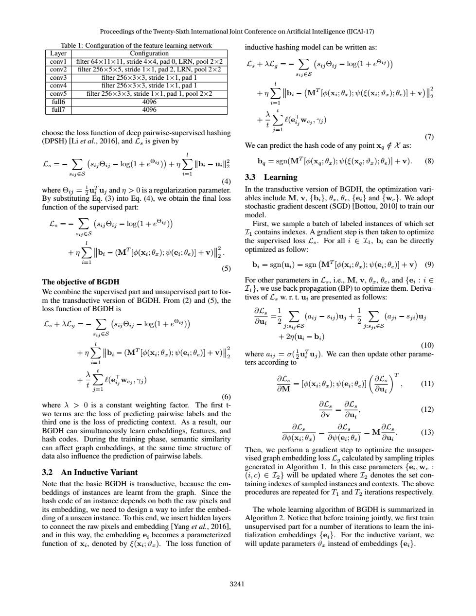
Proceedings of the Twenty-Sixth International Joint Conference on Artificial Intelligence(IJCAI-17) Table 1:Configuration of the feature learning network inductive hashing model can be written as: Layer Configuration convl filter64×11×1l,stride4×4,pad0,LRN,pool2×2 conv2 filter 256x5x5,stride 1x1,pad 2,LRN,pool 2x2 c。+λcg=-∑(8,6j-log(1+e9)月 conv3 filter256×3×3,stride1×l,padl 845∈S conv4 filter256x3×3,stride1×1,padI conv5 filter256x3×3,stride1x1,pad1,pool2×2 +n∑Ilb,-(MP[(x;0)片(5(x;0z):0e月+v)l full6 4096 i=1 full7 4096 ∑ewl choose the loss function of deep pairwise-supervised hashing (DPSH)[Li et al.,2016],and Cs is given by (7) We can predict the hash code of any point xas: C。=-∑(s,6-log(1+e9)+n∑Ib-ul3 ba sgn(M [o(xg:0);(E(xg;v);0e)]+v). (8) 8y∈S i=l (4) 3.3 Learning where j=uuj and n>0 is a regularization parameter. In the transductive version of BGDH,the optimization vari- By substituting Eq.(3)into Eg.(4),we obtain the final loss ables include M,v.[bi},0r,0e,fei}and {we}.We adopt function of the supervised part: stochastic gradient descent(SGD)[Bottou,2010]to train our model. c=-∑ (s6-log(1+e9)】 First,we sample a batch of labeled instances of which set 8时∈S I contains indexes.A gradient step is then taken to optimize the supervised loss Cs.For all i Z1,bi can be directly +b:-(MT[(x:0):(e::0c)]+v)2 optimized as follow: i=1 (5) bi=sgn(ui)=sgn (MT [o(xi;0);u(e;:0e)]+v)(9) The objective of BGDH For other parameters in Cs,i.e.,M,v,0r,e,and fei:iE We combine the supervised part and unsupervised part to for- I1},we use back propagation(BP)to optimize them.Deriva- m the transductive version of BGDH.From(2)and(5),the tives of Cs w.r.t.ui are presented as follows: loss function of BGDH is OC.=1 1 C.+=->e-log(1+e0u)) Oui 2 ∑(a-s4+2∑(a-s叫 j:84y∈S j:8∈S 84∈S +2m(u-b) (10) +n∑lb,-(MP(x;0z(e:9e】+v)l where aij=a(uuj).We can then update other parame- i=1 ters according to +∑em OC (11) j=1 i=[(x;0)片(e:0e】 (6) where A >0 is a constant weighting factor.The first t- ot._OC. wo terms are the loss of predicting pairwise labels and the (12) third one is the loss of predicting context.As a result,our BGDH can simultaneously learn embeddings,features,and 8Cs OCs hash codes.During the training phase,semantic similarity 3o(x:0)Ov(ei;0e) =MOC, u (13) can affect graph embeddings,at the same time structure of Then,we perform a gradient step to optimize the unsuper- data also influence the prediction of pairwise labels. vised graph embedding loss Ca calculated by sampling triples 3.2 An Inductive Variant generated in Algorithm 1.In this case parameters fei,we (i,c)E Z2}will be updated where Z2 denotes the set con- Note that the basic BGDH is transductive,because the em- taining indexes of sampled instances and contexts.The above beddings of instances are learnt from the graph.Since the procedures are repeated for T1 and T2 iterations respectively. hash code of an instance depends on both the raw pixels and its embedding,we need to design a way to infer the embed- The whole learning algorithm of BGDH is summarized in ding of a unseen instance.To this end,we insert hidden layers Algorithm 2.Notice that before training jointly,we first train to connect the raw pixels and embedding [Yang et al.,2016] unsupervised part for a number of iterations to learn the ini- and in this way,the embedding e;becomes a parameterized tialization embeddings [e).For the inductive variant,we function of xi,denoted by (xi;).The loss function of will update parameters instead of embeddings [ei}. 3241Table 1: Configuration of the feature learning network Layer Configuration conv1 filter 64×11×11, stride 4×4, pad 0, LRN, pool 2×2 conv2 filter 256×5×5, stride 1×1, pad 2, LRN, pool 2×2 conv3 filter 256×3×3, stride 1×1, pad 1 conv4 filter 256×3×3, stride 1×1, pad 1 conv5 filter 256×3×3, stride 1×1, pad 1, pool 2×2 full6 4096 full7 4096 choose the loss function of deep pairwise-supervised hashing (DPSH) [Li et al., 2016], and Ls is given by Ls = − X sij∈S ￾ sijΘij − log(1 + e Θij )
+ η X l i=1 kbi − uik 2 2 (4) where Θij = 1 2 u T i uj and η > 0 is a regularization parameter. By substituting Eq. (3) into Eq. (4), we obtain the final loss function of the supervised part: Ls = − X sij∈S ￾ sijΘij − log(1 + e Θij )
+ η X l i=1 bi − (MT [φ(xi ; θx); ψ(ei ; θe)] + v) 2 2 . (5) The objective of BGDH We combine the supervised part and unsupervised part to for￾m the transductive version of BGDH. From (2) and (5), the loss function of BGDH is Ls + λLg = − X sij∈S ￾ sijΘij − log(1 + e Θij )
+ η X l i=1 bi − (MT [φ(xi ; θx); ψ(ei ; θe)] + v) 2 2 + λ t Xt j=1 `(e > ijwcj , γj ) (6) where λ > 0 is a constant weighting factor. The first t￾wo terms are the loss of predicting pairwise labels and the third one is the loss of predicting context. As a result, our BGDH can simultaneously learn embeddings, features, and hash codes. During the training phase, semantic similarity can affect graph embeddings, at the same time structure of data also influence the prediction of pairwise labels. 3.2 An Inductive Variant Note that the basic BGDH is transductive, because the em￾beddings of instances are learnt from the graph. Since the hash code of an instance depends on both the raw pixels and its embedding, we need to design a way to infer the embed￾ding of a unseen instance. To this end, we insert hidden layers to connect the raw pixels and embedding [Yang et al., 2016], and in this way, the embedding ei becomes a parameterized function of xi , denoted by ξ(xi ; ϑx). The loss function of inductive hashing model can be written as: Ls + λLg = − X sij∈S ￾ sijΘij − log(1 + e Θij )
+ η X l i=1 bi − ￾MT [φ(xi ; θx); ψ(ξ(xi ; ϑx); θe)] + v
2 2 + λ t Xt j=1 `(e > ijwcj , γj ) (7) We can predict the hash code of any point xq ∈ X/ as: bq = sgn(MT [φ(xq; θx); ψ(ξ(xq; ϑx); θe)] + v). (8) 3.3 Learning In the transductive version of BGDH, the optimization vari￾ables include M, v, {bi}, θx, θe, {ei} and {wc}. We adopt stochastic gradient descent (SGD) [Bottou, 2010] to train our model. First, we sample a batch of labeled instances of which set I1 contains indexes. A gradient step is then taken to optimize the supervised loss Ls. For all i ∈ I1, bi can be directly optimized as follow: bi = sgn(ui) = sgn ￾MT [φ(xi ; θx); ψ(ei ; θe)] + v
(9) For other parameters in Ls, i.e., M, v, θx, θe, and {ei : i ∈ I1}, we use back propagation (BP) to optimize them. Deriva￾tives of Ls w. r. t. ui are presented as follows: ∂Ls ∂ui = 1 2 X j:sij∈S (aij − sij )uj + 1 2 X j:sji∈S (aji − sji)uj + 2η(ui − bi) (10) where aij = σ( 1 2 u T i uj ). We can then update other parame￾ters according to ∂Ls ∂M = [φ(xi ; θx); ψ(ei ; θe)]  ∂Ls ∂ui T , (11) ∂Ls ∂v = ∂Ls ∂ui , (12) ∂Ls ∂φ(xi ; θx) = ∂Ls ∂ψ(ei ; θe) = M ∂Ls ∂ui . (13) Then, we perform a gradient step to optimize the unsuper￾vised graph embedding loss Lg calculated by sampling triples generated in Algorithm 1. In this case parameters {ei , wc : (i, c) ∈ I2} will be updated where I2 denotes the set con￾taining indexes of sampled instances and contexts. The above procedures are repeated for T1 and T2 iterations respectively. The whole learning algorithm of BGDH is summarized in Algorithm 2. Notice that before training jointly, we first train unsupervised part for a number of iterations to learn the ini￾tialization embeddings {ei}. For the inductive variant, we will update parameters ϑx instead of embeddings {ei}. Proceedings of the Twenty-Sixth International Joint Conference on Artificial Intelligence (IJCAI-17) 3241