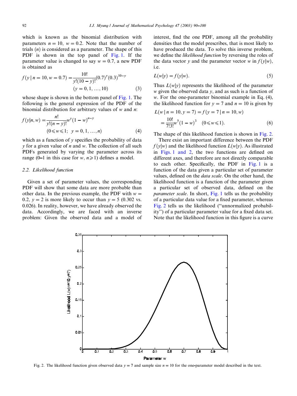
92 1J.Myung I Journal of Mathematical Psychology 47(2003)90-100 which is known as the binomial distribution with interest,find the one PDF,among all the probability parameters n=10,w=0.2.Note that the number of densities that the model prescribes,that is most likely to trials(n)is considered as a parameter.The shape of this have produced the data.To solve this inverse problem, PDF is shown in the top panel of Fig.1.If the we define the likelihood function by reversing the roles of parameter value is changed to say w=0.7,a new PDF the data vector y and the parameter vector w in f(yw), is obtained as i.e. 10川 f0yln=10,w=0.7)= 10-70.7y(0.3)10- L(wly)=f(ylw). (5) 0=0,1,,10) (3) Thus L(wly)represents the likelihood of the parameter w given the observed data y,and as such is a function of whose shape is shown in the bottom panel of Fig.1.The w.For the one-parameter binomial example in Eq.(4), following is the general expression of the PDF of the the likelihood function for y =7 and n=10 is given by binomial distribution for arbitrary values of w and n: L(w|n=10,y=7)=fy=7|n=10,w) n! f6a,w）=-n"(1-w =73n7(1-w320≤w≤1). 101 (6) (0≤w≤1；y=0,1,,n) (4) The shape of this likelihood function is shown in Fig.2. which as a function ofy specifies the probability of data There exist an important difference between the PDF y for a given value of n and w.The collection of all such f(yw)and the likelihood function L(wly).As illustrated PDFs generated by varying the parameter across its in Figs.I and 2,the two functions are defined on range (0-1 in this case for w,n1)defines a model. different axes,and therefore are not directly comparable to each other.Specifically,the PDF in Fig.I is a 2.2.Likelihood function function of the data given a particular set of parameter values,defined on the data scale.On the other hand,the Given a set of parameter values,the corresponding likelihood function is a function of the parameter given PDF will show that some data are more probable than a particular set of observed data,defined on the other data.In the previous example,the PDF with w= parameter scale.In short,Fig.I tells us the probability 0.2,y=2 is more likely to occur than y=5(0.302 vs. of a particular data value for a fixed parameter,whereas 0.026).In reality,however,we have already observed the Fig.2 tells us the likelihood ("unnormalized probabil- data.Accordingly,we are faced with an inverse ity")of a particular parameter value for a fixed data set. problem:Given the observed data and a model of Note that the likelihood function in this figure is a curve 0.35 0.3 0.25 0.2 0.15 0 0.05 0 0.1 2 030,4650.日070a Parameter w Fig.2.The likelihood function given observed data y=7 and sample size n=10 for the one-parameter model described in the textwhich is known as the binomial distribution with parameters n ¼ 10; w ¼ 0:2: Note that the number of trials ðnÞ is considered as a parameter. The shape of this PDF is shown in the top panel of Fig. 1. If the parameter value is changed to say w ¼ 0:7; a new PDF is obtained as fðy j n ¼ 10; w ¼ 0:7Þ ¼ 10! y!ð10  yÞ! ð0:7Þ y ð0:3Þ 10y ðy ¼ 0; 1;y; 10Þ ð3Þ whose shape is shown in the bottom panel of Fig. 1. The following is the general expression of the PDF of the binomial distribution for arbitrary values of w and n: fðyjn; wÞ ¼ n! y!ðn  yÞ! wy ð1  wÞ ny ð0pwp1; y ¼ 0; 1;y; nÞ ð4Þ which as a function of y specifies the probability of data y for a given value of n and w: The collection of all such PDFs generated by varying the parameter across its range (0–1 in this case for w; nX1) defines a model. 2.2. Likelihood function Given a set of parameter values, the corresponding PDF will show that some data are more probable than other data. In the previous example, the PDF with w ¼ 0:2; y ¼ 2 is more likely to occur than y ¼ 5 (0.302 vs. 0.026). In reality, however, we have already observed the data. Accordingly, we are faced with an inverse problem: Given the observed data and a model of interest, find the one PDF, among all the probability densities that the model prescribes, that is most likely to have produced the data. To solve this inverse problem, we define the likelihood function by reversing the roles of the data vector y and the parameter vector w in fðyjwÞ; i.e. LðwjyÞ ¼ fðyjwÞ: ð5Þ Thus LðwjyÞ represents the likelihood of the parameter w given the observed data y; and as such is a function of w: For the one-parameter binomial example in Eq. (4), the likelihood function for y ¼ 7 and n ¼ 10 is given by Lðw j n ¼ 10; y ¼ 7Þ ¼ fðy ¼ 7 j n ¼ 10; wÞ ¼ 10! 7!3! w7 ð1  wÞ 3 ð0pwp1Þ: ð6Þ The shape of this likelihood function is shown in Fig. 2. There exist an important difference between the PDF fðyjwÞ and the likelihood function LðwjyÞ: As illustrated in Figs. 1 and 2, the two functions are defined on different axes, and therefore are not directly comparable to each other. Specifically, the PDF in Fig. 1 is a function of the data given a particular set of parameter values, defined on the data scale. On the other hand, the likelihood function is a function of the parameter given a particular set of observed data, defined on the parameter scale. In short, Fig. 1 tells us the probability of a particular data value for a fixed parameter, whereas Fig. 2 tells us the likelihood (‘‘unnormalized probabil￾ity’’) of a particular parameter value for a fixed data set. Note that the likelihood function in this figure is a curve Fig. 2. The likelihood function given observed data y ¼ 7 and sample size n ¼ 10 for the one-parameter model described in the text. 92 I.J. Myung / Journal of Mathematical Psychology 47 (2003) 90–100