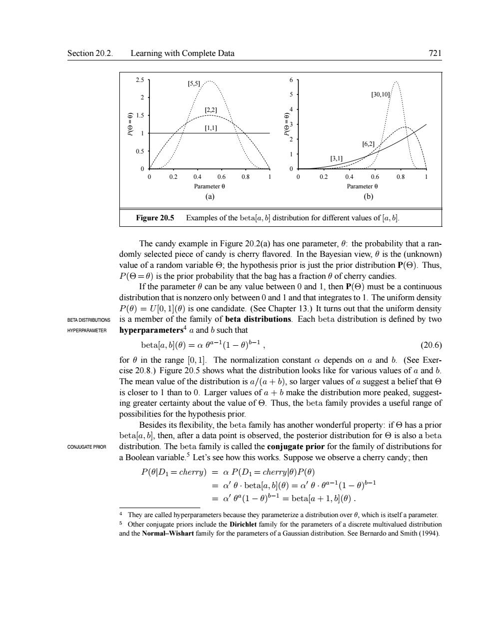
Section 20.2.Learning with Complete Data 721 25 5,1 6 30,10 22 15 621 0.5 0.40.6 0.8 02 0.4 0.6 0.8 Para (a) (b) Figure20.5 Examples of the beta distribution for different values of The candy example in Figure 202(a)has one meter,:the probability that arar domly selected red In the Ba an dis tha lue of a ra ariable the h h P S P just th rdistribution P().Thus P(=0)is the pric probab ility th an value b ag has a ontinuous that zero only o and 1 and that ir tegratest T e uniform one ca s a member f Each tion is defined by two betala,bl(0)=a0a-1(1-0)5-1, (20.6) for 0 in the range 0,1].The normalization constant a depends on a and b.(See Exer- cise 20.8.)Figure 20.5 shows what the distribution looks like for various values of a and b. The mean value of the distribution is a/(ab),so larger values of a suggest a belief that is closer to I than to 0.Larger values ofa+b make the distribution more peaked,suggest- ing greater certainty about the value of Thus,the beta family provides a useful range of possibilities for the hypothesis prior. Besides its flexibility.the beta family has another wonderful pr rty if has a nrior betathneroird.the posterora CONJUGATE PROR distribution.The beta family is called the conjugate prior for the family of distributions for a Boolean variable.5 Let's see how this works.Suppose we observe a cherry candy.then P(D1=cherry)=a P(D1=cherryl0)P(0) =a'0.betafa,](0)=a'0.0-1(1-0)-1 =a'(1-)b betala +1,(0). 4They are called hyperparameters beca Smith (19)Section 20.2. Learning with Complete Data 721 0 0.5 1 1.5 2 2.5 0 0.2 0.4 0.6 0.8 1 P(Θ = θ) Parameter θ [1,1] [2,2] [5,5] 0 1 2 3 4 5 6 0 0.2 0.4 0.6 0.8 1 P(Θ = θ) Parameter θ [3,1] [6,2] [30,10] (a) (b) Figure 20.5 Examples of the beta[a, b] distribution for different values of [a, b]. The candy example in Figure 20.2(a) has one parameter, θ: the probability that a ran￾domly selected piece of candy is cherry flavored. In the Bayesian view, θ is the (unknown) value of a random variable Θ; the hypothesis prior is just the prior distribution P(Θ). Thus, P(Θ = θ) is the prior probability that the bag has a fraction θ of cherry candies. If the parameter θ can be any value between 0 and 1, then P(Θ) must be a continuous distribution that is nonzero only between 0 and 1 and that integratesto 1. The uniform density P(θ) = U[0, 1](θ) is one candidate. (See Chapter 13.) It turns out that the uniform density BETA DISTRIBUTIONS is a member of the family of beta distributions. Each beta distribution is defined by two hyperparameters4 HYPERPARAMETER a and b such that beta[a, b](θ) = α θ a−1 (1 − θ) b−1 , (20.6) for θ in the range [0, 1]. The normalization constant α depends on a and b. (See Exer￾cise 20.8.) Figure 20.5 shows what the distribution looks like for various values of a and b. The mean value of the distribution is a/(a + b), so larger values of a suggest a belief that Θ is closer to 1 than to 0. Larger values of a + b make the distribution more peaked, suggest￾ing greater certainty about the value of Θ. Thus, the beta family provides a useful range of possibilities for the hypothesis prior. Besides its flexibility, the beta family has another wonderful property: if Θ has a prior beta[a, b], then, after a data point is observed, the posterior distribution for Θ is also a beta CONJUGATE PRIOR distribution. The beta family is called the conjugate prior for the family of distributions for a Boolean variable.5 Let’s see how this works. Suppose we observe a cherry candy; then P(θ|D1 = cherry) = α P(D1 = cherry|θ)P(θ) = α 0 θ · beta[a, b](θ) = α 0 θ · θ a−1 (1 − θ) b−1 = α 0 θ a (1 − θ) b−1 = beta[a + 1, b](θ) . 4 They are called hyperparameters because they parameterize a distribution over θ, which is itself a parameter. 5 Other conjugate priors include the Dirichlet family for the parameters of a discrete multivalued distribution and the Normal–Wishart family for the parameters of a Gaussian distribution. See Bernardo and Smith (1994)