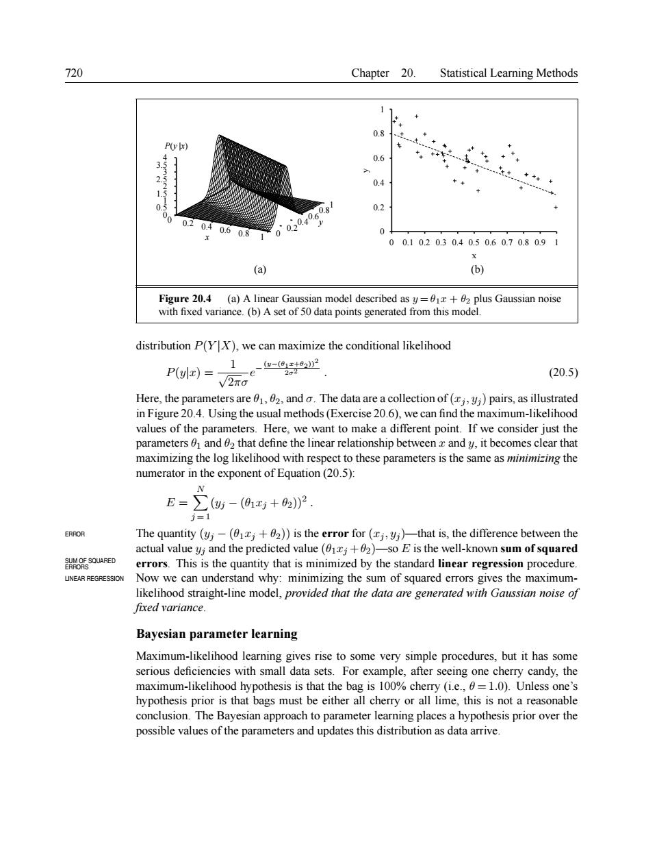
720 Chapter 20.Statistical Learning Methods 11 0.6 0.4 02 0.6 0 00.102030.40.50.60.70.80.9 (a) sian model described asy+2 plus Gaussian noise distribution P(YX),we can maximize the conditional likelihood 1 (20.5) Here,the parameters are02.and.The data are a collection of()pairs,as illustrated in Figure 20.4.Using the usual methods(Exercise 20.6),we can find the maximum-likelihood values of the parameters.Here,we want to make a different point.If we consider just the parameters and 02 that define the linear relationship betweenz andy,it becomes clear that maximizing the log likelihood with respect to these parameters is the same as minimizing the numerator in the exponent of Equation(20.5): E=∑防-01+2P =1 The qntty(y一4巧土》is theeroor(,%hats.thefr benthe and the dicted value :+02 Im ofs SUM OE SOURPED tity that is min zed by y the standard lin regr ssio edur INEAR REGRESSION ing the model.pro ided t squared he ght-line sia noise fixed variance. Bayesian parameter learning Maximum-likelihood learning gives rise to some very simple procedures.but it has some serious deficiencies with small data sets.For example,after seeing one cherry candy,the maximum-likelihood hypothesis is that the bag is 100%cherry (i.e.,=1.0).Unless one's hypothesis prior is that bags must be either all cherry or all lime,this is not a reasonable conclusion.The Bayesian approach to parameter learning places a hypothesis prior over the possible values of the parameters and updates this distribution as data arrive. 720 Chapter 20. Statistical Learning Methods 0 0.2 0.4 0.6 0.8 x 1 0 0.20.40.60.81 y 0 0.5 1 1.5 2 2.5 3 3.5 4 P(y |x) 0 0.2 0.4 0.6 0.8 1 0 0.1 0.2 0.3 0.4 0.5 0.6 0.7 0.8 0.9 1 y x (a) (b) Figure 20.4 (a) A linear Gaussian model described as y = θ1x + θ2 plus Gaussian noise with fixed variance. (b) A set of 50 data points generated from this model. distribution P(Y |X), we can maximize the conditional likelihood P(y|x) = 1 √ 2πσ e − (y−(θ1x+θ2))2 2σ2 . (20.5) Here, the parameters are θ1, θ2, and σ. The data are a collection of (xj , yj ) pairs, as illustrated in Figure 20.4. Using the usual methods(Exercise 20.6), we can find the maximum-likelihood values of the parameters. Here, we want to make a different point. If we consider just the parameters θ1 and θ2 that define the linear relationship between x and y, it becomes clear that maximizing the log likelihood with respect to these parameters is the same as minimizing the numerator in the exponent of Equation (20.5): E = X N j = 1 (yj − (θ1xj + θ2))2 . ERROR The quantity (yj − (θ1xj + θ2)) is the error for (xj , yj )—that is, the difference between the actual value yj and the predicted value (θ1xj +θ2)—so E is the well-known sum of squared errors. This is the quantity that is minimized by the standard linear regression procedure. SUM OF SQUARED ERRORS LINEAR REGRESSION Now we can understand why: minimizing the sum of squared errors gives the maximum￾likelihood straight-line model, provided that the data are generated with Gaussian noise of fixed variance. Bayesian parameter learning Maximum-likelihood learning gives rise to some very simple procedures, but it has some serious deficiencies with small data sets. For example, after seeing one cherry candy, the maximum-likelihood hypothesis is that the bag is 100% cherry (i.e., θ = 1.0). Unless one’s hypothesis prior is that bags must be either all cherry or all lime, this is not a reasonable conclusion. The Bayesian approach to parameter learning places a hypothesis prior over the possible values of the parameters and updates this distribution as data arrive