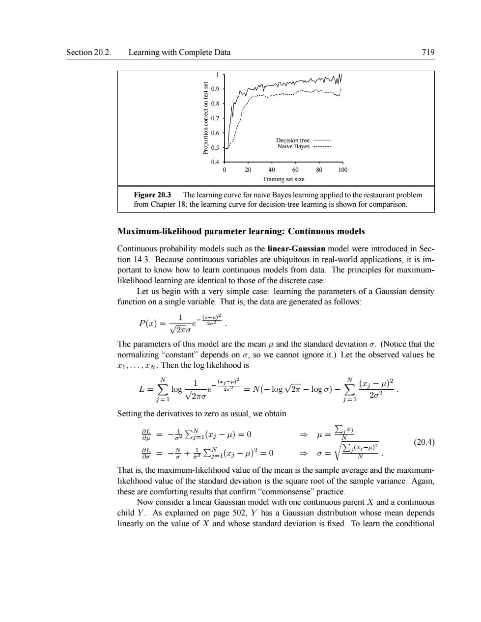
Section 20.2.Learning with Complete Data 719 08 07 20 40 60 80100 Trainine set size Figure20.3 The learning curve for naive Bayes learning applied to the restaurant problem from Chapter 18;the learning curve for decision-tree learning is shown for comparison. Maximum-likelihood parameter learning:Continuous models Continuous probability models such as the linear-Gaussian model were introduced in Sec. portant to know how to leamn continugus models from data likelihood learning are identical to those of the discrete case I et us he in with a very simple case:learning the arameters of a Gaussian density function on a single variable.That is.the data are g enerated as follows: P(x)= √2 The parameters of this model are the mean u and the standard deviation a (Notice that the normalizing"constant"depends on o,so we cannot ignore it.)Let the observed values be N.Then the log likelihood is 。e 1 -=N(-log v2-logo)- X(-)2 122 Setting the derivatives to zero as usual,we obtain =-（红-4=0 →“= →=V②色9 (20.4) 0=-￥+÷∑1(-4)2=0 That is,the maximum-likelihood value of the mean is the sample average and the maximum- likelihood value of the standard deviation is the square root of the sample variance.Again. these are comforting results that confirm"commor Now consider a linear Gaussian model with one continuous parent X and a continuous child Y.As explained on page 502.Y has a Gaussian distribution whose mean depends linearly on the value of X and whose standard deviation is fixed.To learn the conditionalSection 20.2. Learning with Complete Data 719 0.4 0.5 0.6 0.7 0.8 0.9 1 0 20 40 60 80 100 Proportion correct on test set Training set size Decision tree Naive Bayes Figure 20.3 The learning curve for naive Bayes learning applied to the restaurant problem from Chapter 18; the learning curve for decision-tree learning is shown for comparison. Maximum-likelihood parameter learning: Continuous models Continuous probability models such as the linear-Gaussian model were introduced in Sec￾tion 14.3. Because continuous variables are ubiquitous in real-world applications, it is im￾portant to know how to learn continuous models from data. The principles for maximum￾likelihood learning are identical to those of the discrete case. Let us begin with a very simple case: learning the parameters of a Gaussian density function on a single variable. That is, the data are generated as follows: P(x) = 1 √ 2πσ e − (x−µ) 2 2σ2 . The parameters of this model are the mean µ and the standard deviation σ. (Notice that the normalizing “constant” depends on σ, so we cannot ignore it.) Let the observed values be x1, . . . , xN . Then the log likelihood is L = X N j = 1 log 1 √ 2πσ e − (xj−µ) 2 2σ2 = N(− log √ 2π − log σ) − X N j = 1 (xj − µ) 2 2σ2 . Setting the derivatives to zero as usual, we obtain ∂L ∂µ = − 1 σ2 PN j=1(xj − µ) = 0 ⇒ µ = P j xj N ∂L ∂σ = − N σ + 1 σ3 PN j=1(xj − µ) 2 = 0 ⇒ σ = rP j (xj−µ) 2 N . (20.4) That is, the maximum-likelihood value of the mean is the sample average and the maximum￾likelihood value of the standard deviation is the square root of the sample variance. Again, these are comforting results that confirm “commonsense” practice. Now consider a linear Gaussian model with one continuous parent X and a continuous child Y . As explained on page 502, Y has a Gaussian distribution whose mean depends linearly on the value of X and whose standard deviation is fixed. To learn the conditional