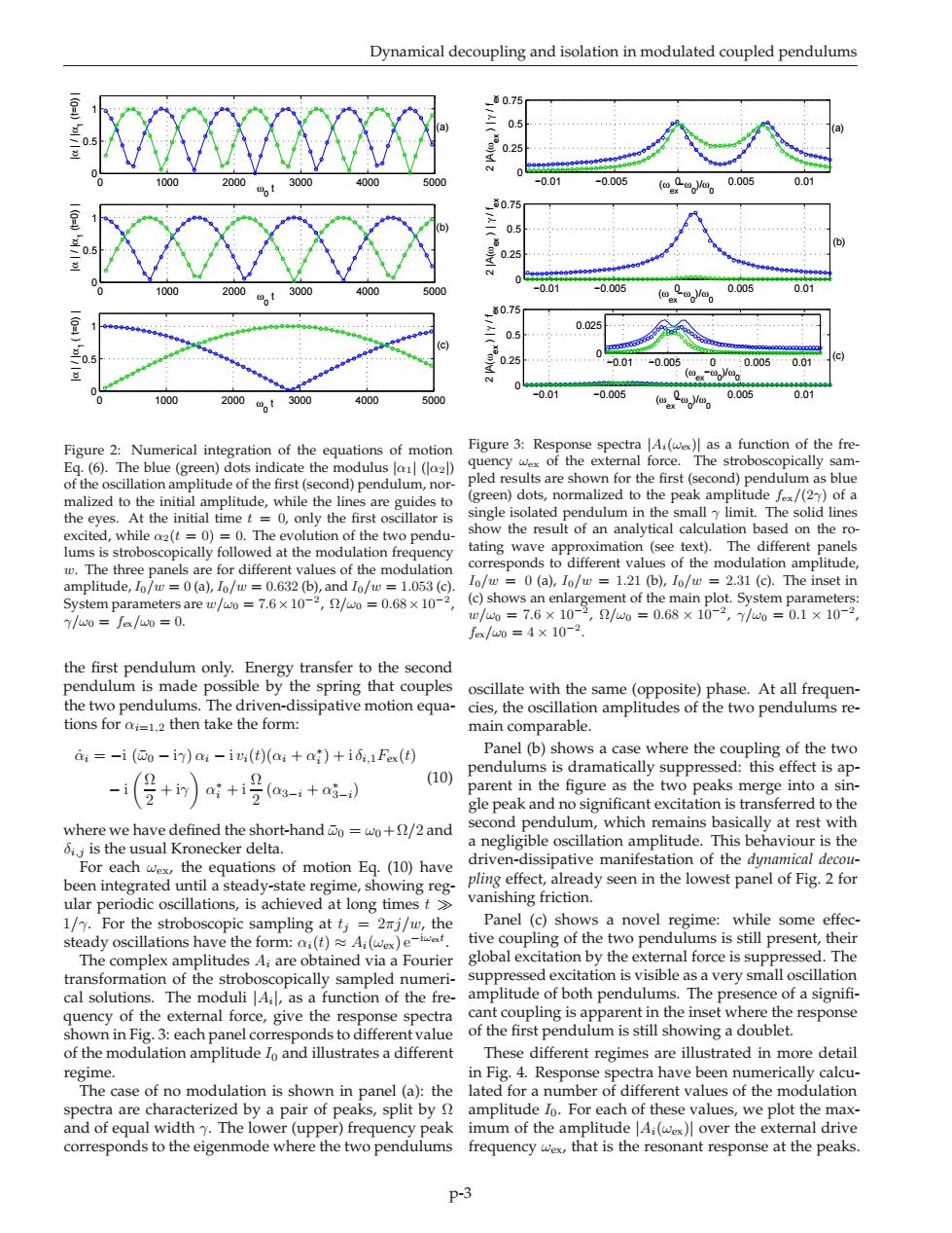
Dynamical decoupling and isolation in modulated coupled pendulums 0.7 000 0.25 -0.01-005 001 0.005 e,%00o6 0.01 0.025 0.5 025 00050 1000 200, 3000 4000 lA)as a function of the fr Figure 2:Numerical integration of the equations of motion ond)pendulum,no )d normalized to the peak amplit tudef(2)of a the line are guides nof the two pendu olatedpe imit. The solid (see text).The different p e for diffo 0a 0=1.21b 231().The in 2/w0=0.68X1 (c)shows an er gm=4×10-2 transfer to the second tions for2 then take the form: main comparable. as=-i(0-)a;-iv(t)(ai+ai)+i6i..Fex(t) Panel (b)show a case where the c of the twe pendulums is dramatically suppr sed this effect isap -i(侵+n）a+号ag-4+a-) (10) peaks merge into a sir sign nt exc 1 where we have defined the short-hand o=wo+/2 and at rest is the usual Kronecker delta. a negligible oscillation amplitude.This behaviour is the or each the equations of motion Eq.(10)have driven-dissipative manifestation of the dynamical decou inadyseen in the lowest panel o 1/.For the stroboscopic sampling at t 2rj/w,the Panel sho th s a novel regime while some efe steady oscillations have the form:(t)A)e lobalexcitation hy the exter nal force is su Ai are ained via a Fourier sed.The cal solutions.The moduli as a function of the fre- amplitude of both pendulums.The pre esence of a signit 好 erent regimes re The case of no modulation is shown in panel (a):the ks,split by amplitude lo.For each of these values,we plot the max- The imum of the amp Ai(wex)over the correspo se at the peaks p-3 Dynamical decoupling and isolation in modulated coupled pendulums 0 1000 2000 3000 4000 5000 0 0.5 1 ω0 t |α | / |α 1 (t=0) | 0 1000 2000 3000 4000 5000 0 0.5 1 ω0 t |α | / |α 1 (t=0) | 0 1000 2000 3000 4000 5000 0 0.5 1 ω0 t |α | / |α 1 ( t=0) | (c) (b) (a) Figure 2: Numerical integration of the equations of motion Eq. (6). The blue (green) dots indicate the modulus |α1| (|α2|) of the oscillation amplitude of the first (second) pendulum, nor￾malized to the initial amplitude, while the lines are guides to the eyes. At the initial time t = 0, only the first oscillator is excited, while α2(t = 0) = 0. The evolution of the two pendu￾lums is stroboscopically followed at the modulation frequency w. The three panels are for different values of the modulation amplitude, I0/w = 0 (a), I0/w = 0.632 (b), and I0/w = 1.053 (c). System parameters are w/ω0 = 7.6×10−2 , Ω/ω0 = 0.68×10−2 , γ/ω0 = fex/ω0 = 0. the first pendulum only. Energy transfer to the second pendulum is made possible by the spring that couples the two pendulums. The driven-dissipative motion equa￾tions for αi=1,2 then take the form: α˙ i = −i (¯ω0 − iγ) αi − i vi(t)(αi + α ∗ i ) + i δi,1Fex(t) − i  Ω 2 + iγ  α ∗ i + i Ω 2 (α3−i + α ∗ 3−i ) (10) where we have defined the short-hand ω¯0 = ω0+Ω/2 and δi,j is the usual Kronecker delta. For each ωex, the equations of motion Eq. (10) have been integrated until a steady-state regime, showing reg￾ular periodic oscillations, is achieved at long times t ≫ 1/γ. For the stroboscopic sampling at tj = 2πj/w, the steady oscillations have the form: αi(t) ≈ Ai(ωex) e−iωext . The complex amplitudes Ai are obtained via a Fourier transformation of the stroboscopically sampled numeri￾cal solutions. The moduli |Ai |, as a function of the fre￾quency of the external force, give the response spectra shown in Fig. 3: each panel corresponds to different value of the modulation amplitude I0 and illustrates a different regime. The case of no modulation is shown in panel (a): the spectra are characterized by a pair of peaks, split by Ω and of equal width γ. The lower (upper) frequency peak corresponds to the eigenmode where the two pendulums −0.01 −0.005 0 0.005 0.01 0 0.25 0.5 0.75 (ωex −ω0 )/ω0 2 |A(ωex ) | γ / fex −0.01 −0.005 0 0.005 0.01 0 0.25 0.5 0.75 (ωex −ω0 )/ω0 2 |A(ωex ) | γ / fex −0.01 −0.005 0 0.005 0.01 0 0.25 0.5 0.75 (ωex −ω0 )/ω0 2 |A(ωex ) | γ / fex −0.01 −0.005 0 0.005 0.01 0 0.025 (ωex −ω0 )/ω0 (a) (c) (b) Figure 3: Response spectra |Ai(ωex)| as a function of the fre￾quency ωex of the external force. The stroboscopically sam￾pled results are shown for the first (second) pendulum as blue (green) dots, normalized to the peak amplitude fex/(2γ) of a single isolated pendulum in the small γ limit. The solid lines show the result of an analytical calculation based on the ro￾tating wave approximation (see text). The different panels corresponds to different values of the modulation amplitude, I0/w = 0 (a), I0/w = 1.21 (b), I0/w = 2.31 (c). The inset in (c) shows an enlargement of the main plot. System parameters: w/ω0 = 7.6 × 10−2 , Ω/ω0 = 0.68 × 10−2 , γ/ω0 = 0.1 × 10−2 , fex/ω0 = 4 × 10−2 . oscillate with the same (opposite) phase. At all frequen￾cies, the oscillation amplitudes of the two pendulums re￾main comparable. Panel (b) shows a case where the coupling of the two pendulums is dramatically suppressed: this effect is ap￾parent in the figure as the two peaks merge into a sin￾gle peak and no significant excitation is transferred to the second pendulum, which remains basically at rest with a negligible oscillation amplitude. This behaviour is the driven-dissipative manifestation of the dynamical decou￾pling effect, already seen in the lowest panel of Fig. 2 for vanishing friction. Panel (c) shows a novel regime: while some effec￾tive coupling of the two pendulums is still present, their global excitation by the external force is suppressed. The suppressed excitation is visible as a very small oscillation amplitude of both pendulums. The presence of a signifi- cant coupling is apparent in the inset where the response of the first pendulum is still showing a doublet. These different regimes are illustrated in more detail in Fig. 4. Response spectra have been numerically calcu￾lated for a number of different values of the modulation amplitude I0. For each of these values, we plot the max￾imum of the amplitude |Ai(ωex)| over the external drive frequency ωex, that is the resonant response at the peaks. p-3