正在加载图片...

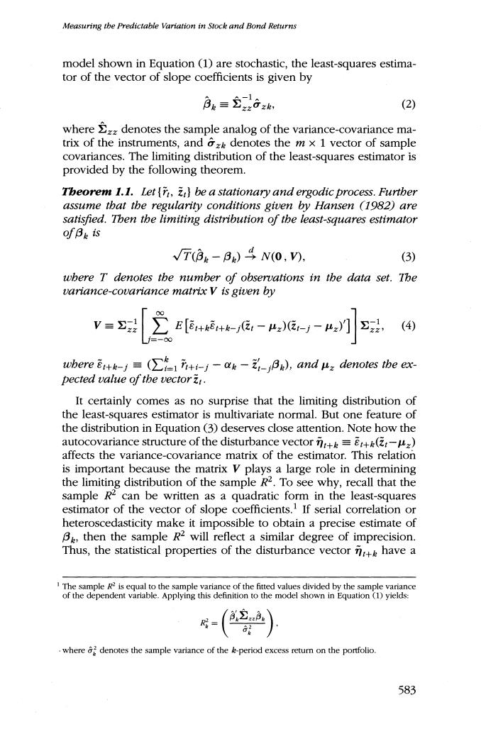
Measuring the Predictable Variation in Stock and Bond Returns model shown in Equation (1)are stochastic,the least-squares estima- tor of the vector of slope coefficients is given by ae=26, (2) wheredenotes the sample analog of the variance-covariance ma- trix of the instruments,and z denotes the m x 1 vector of sample covariances.The limiting distribution of the least-squares estimator is provided by the following theorem. Theorem 1.1.Let(n,be a stationary and ergodic process.Furtber assume that the regularity conditions given by Hansen (1982)are satisfied.Then the limiting distribution of the least-squares estimator ofF。is √T(3。-B)号N(0,V, (3) wbere T denotes the number of observations in the data set.The variance-covariance matrix V is given by 2z2 (④ wbere=(-aB),and u:denotes the ex- pected value of the vector i:. It certainly comes as no surprise that the limiting distribution of the least-squares estimator is multivariate normal.But one feature of the distribution in Equation (3)deserves close attention.Note how the autocovariance structure of the disturbance vector=(-) affects the variance-covariance matrix of the estimator.This relation is important because the matrix V plays a large role in determining the limiting distribution of the sample R2.To see why,recall that the sample R can be written as a quadratic form in the least-squares estimator of the vector of slope coefficients.If serial correlation or heteroscedasticity make it impossible to obtain a precise estimate of Ba,then the sample R2 will reflect a similar degree of imprecision. Thus,the statistical properties of the disturbance vector n+have a The sample R2 is equal to the sample variance of the fitted values divided by the sample variance of the dependent variable.Applying this definition to the model shown in Equation (1)yields: where denotes the sample variance of the k-period excess return on the portfolio. 583