3.2.Context-Aware Masking Table 1.Tasks on VoxCelebl dataset.Here 'O'denotes 'original', We denote the input acoustic features as x.The output feature map "E'denotes 'extended'.and'H'denotes 'hard'. of a selected hidden layer is: #of VoxCeleb1-0 VoxCelebl-E VoxCeleb1-H g(F(x)), (3) Speakers 40 1.251 1.251 Trial pairs 37,611 579,818 550.894 where g()denotes the transformation of the hidden layer and F() denotes the transformation of the layers before the hidden layer. In previous speech enhancement-based methods,the first step is where u is the mean vector and o is the standard deviation vector. to predict enhanced acoustic features,denoted as x.The correspond- ing output feature map of the hidden layer becomes: Following the statistics pooling layer,an FC layer maps the mean and standard deviation vectors into context embedding: 9(F(). (4) e=W3[u,o]+b3, (11) As shown in Figure 1 (b),feature map masking is to apply a ratio where denotes concatenation. mask on the feature map.It is possible to obtain a similar effect with CAM can be applied multiple times to different layers.In our speech enhancement if we can find a mask M that satisfies: experiment,we apply it to the first position-wise FC layer in the vanilla TDNN and the transition layer in each block of D-TDNN. g(F(x)⊙Mxg(F(), (⑤) The context embedding size is half of the output size of the selected hidden layer where denotes element-wise multiplication,and the elements of M can be normalized to the range of(0,1). In the following part,we demonstrate how to estimate a proper 4.EXPERIMENT ratio mask.To achieve this goal,we employ the characteristics of the speaker of interest and noise,which can be derived from an auxiliary 4.1.Dataset context embedding,denoted as e.As shown in Figure 1 (c),we To evaluate the effectiveness of CAM,we conduct experiments on predict the context-aware mask frame by frame: the popular speaker verification dataset VoxCeleb [24].The utter- ances in VoxCeleb are collected from online videos through an auto- F=F(x), (6) mated pipeline and across unconstrained conditions.Thus,there are M.t=o(W2w(WIF.t+e)+b2), (7 both clean and noisy utterances in VoxCeleb. VoxCeleb consists of two subsets,including VoxCelebl and F=g(F(x)⊙M, (8) VoxCeleb2.We use the development set of VoxCeleb2 for training where ()denotes the Sigmoid function,w()denotes the combina- the models,which contains 5,994 speakers.After that,we evaluate the models on VoxCeleb1.As shown in Table 1,there are three tasks tion of ReLU function and BN.M is the predicted ratio mask,M.t and F.denote their t-th frames.F is the feature map after masking. on VoxCelebl,and the last two tasks have more trial pairs. The auxiliary context embedding e serves as a dynamic bias vector that controls the activation threshold. 4.2.Implementation Details In context-aware speech enhancement [19,22],speaker embed- The input features are 80-dimensional log-Mel filter banks extracted ding or noise embedding are extracted by pre-trained embedding over a 25 ms long window for every 10 ms.We also adopt cepstral models.Context-aware masking(CAM),on the other hand,dynam- mean normalization over a 3-second sliding window.All data prepa- ically extracts context embedding.This method does not require ration steps mentioned above are processed in the Kaldi toolkit [25]. extra clean utterance from the speaker of interest as reference.It Data augmentation is also commonly used in training robust automatically finds the main speaker in forwarding propagation. speaker embedding models.Therefore,we adopt similar strategies CAM is designed to recognize a speaker as the main speaker if in [26]to augment data,including simulating reverberation with the any of the following conditions are met:(1)The majority of speech RIR dataset [27].adding noise with the MUSAN dataset [28],and in an utterance comes from this speaker.(2)This speaker's volume changing tempo.We also adopt SpecAugment [29].which randomly is significantly higher than others.Other speakers that appear in masks 0 to 10 frequency channels and 0 to 5 time frames the utterance are called interfering speakers.It is beneficial to omit We implement all models in PyTorch.We refer the reader to [5] the speech of interfering speakers and non-speech noise in speaker and its GitHub page for the detailed structure of D-TDNN.We train verification tasks. all models with angular additive margin softmax (AAM-Softmax) A simple approach to find the main speaker and global non- loss [30].The margin and scaling factor of AAM-Softmax loss are speech noise is to extract an utterance-level embedding.As shown set to 0.25 and 32,respectively.We adopt the stochastic gradient in Figure 1 (c),we extract context embedding based on the input descent(SGD)optimizer,and the mini-batch size is 128.The mo- feature map of the hidden layer.First,we combine all frames with a mentum is 0.95.and the weight decay is 5e-4.We randomly crop a statistics pooling layer: 400-frame sample from each spectrogram when we construct mini- batches.The initial learning rate is 0.01,and we divide the learning rate by 10 at the 120K-th and 180K-th iterations.Training terminates = (9) at the 240K-th iterations. We adopt cosine scoring and adaptive score normalization (AS- Norm)[31]for all models.The imposter cohort consists of the av- t⊙Ft一⊙山 (10) erages of the 22-normalized speaker embeddings of each training speaker.The size of the imposter cohort is 1000.3.2. Context-Aware Masking We denote the input acoustic features as x. The output feature map of a selected hidden layer is: g(F(x)), (3) where g(·) denotes the transformation of the hidden layer and F(·) denotes the transformation of the layers before the hidden layer. In previous speech enhancement-based methods, the first step is to predict enhanced acoustic features, denoted as x˜. The correspond￾ing output feature map of the hidden layer becomes: g(F(x˜)). (4) As shown in Figure 1 (b), feature map masking is to apply a ratio mask on the feature map. It is possible to obtain a similar effect with speech enhancement if we can find a mask M˜ that satisfies: g(F(x))  M˜ ∝ g(F(x˜)), (5) where  denotes element-wise multiplication, and the elements of M˜ can be normalized to the range of (0, 1). In the following part, we demonstrate how to estimate a proper ratio mask. To achieve this goal, we employ the characteristics of the speaker of interest and noise, which can be derived from an auxiliary context embedding, denoted as e. As shown in Figure 1 (c), we predict the context-aware mask frame by frame: F = F(x), (6) M∗t = σ(W> 2 ω(W> 1 F∗t + e) + b2), (7) F˜ = g(F(x))  M, (8) where σ(·) denotes the Sigmoid function, ω(·) denotes the combina￾tion of ReLU function and BN. M is the predicted ratio mask, M∗t and F∗t denote their t-th frames. F˜ is the feature map after masking. The auxiliary context embedding e serves as a dynamic bias vector that controls the activation threshold. In context-aware speech enhancement [19, 22], speaker embed￾ding or noise embedding are extracted by pre-trained embedding models. Context-aware masking (CAM), on the other hand, dynam￾ically extracts context embedding. This method does not require extra clean utterance from the speaker of interest as reference. It automatically finds the main speaker in forwarding propagation. CAM is designed to recognize a speaker as the main speaker if any of the following conditions are met: (1) The majority of speech in an utterance comes from this speaker. (2) This speaker’s volume is significantly higher than others. Other speakers that appear in the utterance are called interfering speakers. It is beneficial to omit the speech of interfering speakers and non-speech noise in speaker verification tasks. A simple approach to find the main speaker and global non￾speech noise is to extract an utterance-level embedding. As shown in Figure 1 (c), we extract context embedding based on the input feature map of the hidden layer. 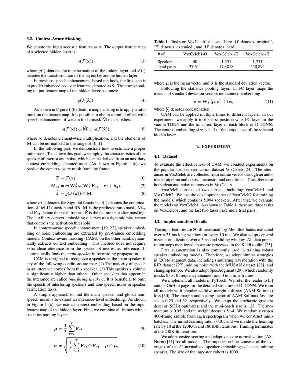First, we combine all frames with a statistics pooling layer: µ = 1 T XT t=1 F∗t, (9) σ = vuut 1 T XT t=1 F∗t  F∗t − µ  µ, (10) Table 1. Tasks on VoxCeleb1 dataset. Here ‘O’ denotes ‘original’, ‘E’ denotes ‘extended’, and ‘H’ denotes ‘hard’. # of VoxCeleb1-O VoxCeleb1-E VoxCeleb1-H Speakers 40 1,251 1,251 Trial pairs 37,611 579,818 550,894 where µ is the mean vector and σ is the standard deviation vector. Following the statistics pooling layer, an FC layer maps the mean and standard deviation vectors into context embedding: e = W> 3 [µ, σ] + b3, (11) where [·] denotes concatenation. CAM can be applied multiple times to different layers. In our experiment, we apply it to the first position-wise FC layer in the vanilla TDNN and the transition layer in each block of D-TDNN. The context embedding size is half of the output size of the selected hidden layer. 4. EXPERIMENT 4.1. Dataset To evaluate the effectiveness of CAM, we conduct experiments on the popular speaker verification dataset VoxCeleb [24]. The utter￾ances in VoxCeleb are collected from online videos through an auto￾mated pipeline and across unconstrained conditions. Thus, there are both clean and noisy utterances in VoxCeleb. VoxCeleb consists of two subsets, including VoxCeleb1 and VoxCeleb2. We use the development set of VoxCeleb2 for training the models, which contains 5,994 speakers. After that, we evaluate the models on VoxCeleb1. As shown in Table 1, there are three tasks on VoxCeleb1, and the last two tasks have more trial pairs. 4.2. Implementation Details The input features are 80-dimensional log-Mel filter banks extracted over a 25 ms long window for every 10 ms. We also adopt cepstral mean normalization over a 3-second sliding window. All data prepa￾ration steps mentioned above are processed in the Kaldi toolkit [25]. Data augmentation is also commonly used in training robust speaker embedding models. Therefore, we adopt similar strategies in [26] to augment data, including simulating reverberation with the RIR dataset [27], adding noise with the MUSAN dataset [28], and changing tempo. We also adopt SpecAugment [29], which randomly masks 0 to 10 frequency channels and 0 to 5 time frames. We implement all models in PyTorch. We refer the reader to [5] and its GitHub page for the detailed structure of D-TDNN. We train all models with angular additive margin softmax (AAM-Softmax) loss [30]. The margin and scaling factor of AAM-Softmax loss are set to 0.25 and 32, respectively. We adopt the stochastic gradient descent (SGD) optimizer, and the mini-batch size is 128. The mo￾mentum is 0.95, and the weight decay is 5e-4. We randomly crop a 400-frame sample from each spectrogram when we construct mini￾batches. The initial learning rate is 0.01, and we divide the learning rate by 10 at the 120K-th and 180K-th iterations. Training terminates at the 240K-th iterations. We adopt cosine scoring and adaptive score normalization (AS￾Norm) [31] for all models. The imposter cohort consists of the av￾erages of the `2-normalized speaker embeddings of each training speaker. The size of the imposter cohort is 1000