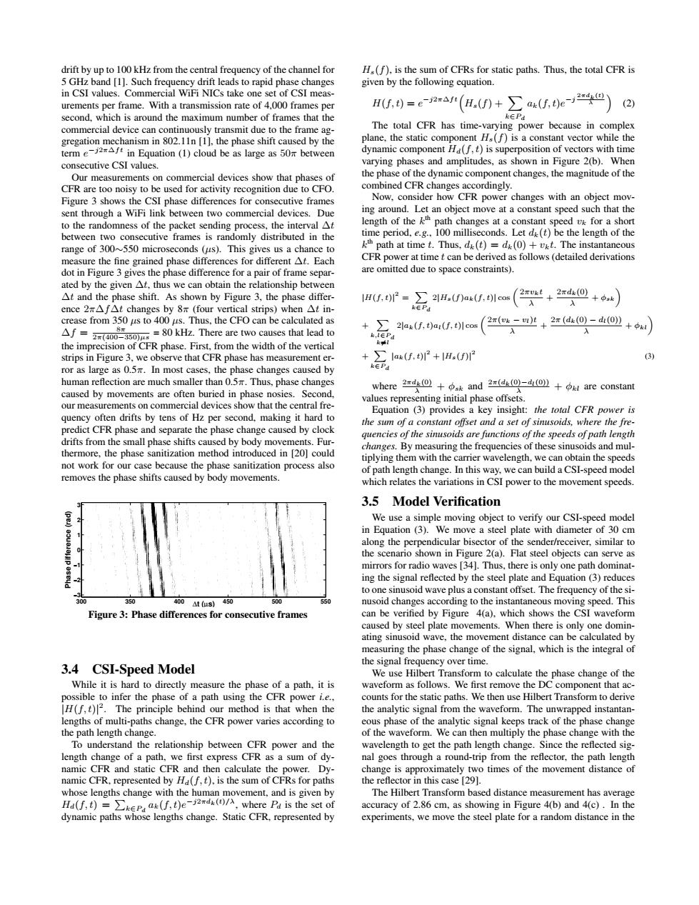
drift by up to 100 kHz from the central frequency of the channel for H.(f).is the sum of CFRs for static paths.Thus,the total CFR is 5 GHz band [1].Such frequency drift leads to rapid phase changes given by the following equation. in CSI values.Commercial WiFi NICs take one set of CSI meas- urements per frame.With a transmission rate of 4,000 frames per H(f,t)=e(H()+>ax(f,t)e (2) second,which is around the maximum number of frames that the kEPd commercial device can continuously transmit due to the frame ag- The total CFR has time-varying power because in complex gregation mechanism in 802.11n [1].the phase shift caused by the plane,the static component H(f)is a constant vector while the term e in Equation(1)cloud be as large as 50 between dynamic component Ha(f,t)is superposition of vectors with time consecutive CSI values. varying phases and amplitudes,as shown in Figure 2(b).When Our measurements on commercial devices show that phases of the phase of the dynamic component changes,the magnitude of the CFR are too noisy to be used for activity recognition due to CFO. combined CFR changes accordingly. Figure 3 shows the CSI phase differences for consecutive frames Now,consider how CFR power changes with an object mov- sent through a WiFi link between two commercial devices.Due ing around.Let an object move at a constant speed such that the to the randomness of the packet sending process,the interval At length of the kth path changes at a constant speed v for a short between two consecutive frames is randomly distributed in the time period,e.g.,100 milliseconds.Let d(t)be the length of the range of 300~550 microseconds (us).This gives us a chance to kth path at time t.Thus,d(t)=dk(0)+vxt.The instantaneous measure the fine grained phase differences for different At.Each CFR power at time t can be derived as follows (detailed derivations dot in Figure 3 gives the phase difference for a pair of frame separ- are omitted due to space constraints). ated by the given At,thus we can obtain the relationship between At and the phase shift.As shown by Figure 3,the phase differ- 1Hf,trP=∑2A.a,圳os(2+2d0+） 入 ence2r△f△t changes by8π(four vertical strips)when△tin- kEPd crease from 350 us to 400 us.Thus,the CFO can be calculated as 2lak(f,t)ai(f,t)l cos /2aos-m+2红(d0）-do+a Af==80 kHz.There are two causes that lead to k,lEPd the imprecision of CFR phase.First,from the width of the vertical k strips in Figure 3,we observe that CFR phase has measurement er- +Iak(f,t2+1H()2 (3) ror as large as 0.5.In most cases,the phase changes caused by kEPd human reflection are much smaller than 0.5m.Thus,phase changes where24@+中kand2红o-4o》+are constant caused by movements are often buried in phase nosies.Second, values representing initial phase offsets. our measurements on commercial devices show that the central fre- Equation (3)provides a key insight:the total CFR power is quency often drifts by tens of Hz per second,making it hard to the sum of a constant offset and a set of sinusoids,where the fre- predict CFR phase and separate the phase change caused by clock quencies of the sinusoids are functions of the speeds of path length drifts from the small phase shifts caused by body movements.Fur- changes.By measuring the frequencies of these sinusoids and mul- thermore,the phase sanitization method introduced in [20]could tiplying them with the carrier wavelength,we can obtain the speeds not work for our case because the phase sanitization process also of path length change.In this way,we can build a CSI-speed model removes the phase shifts caused by body movements. which relates the variations in CSI power to the movement speeds. 3.5 Model Verification We use a simple moving object to verify our CSI-speed model in Equation (3).We move a steel plate with diameter of 30 cm along the perpendicular bisector of the sender/receiver,similar to the scenario shown in Figure 2(a).Flat steel objects can serve as mirrors for radio waves [34].Thus,there is only one path dominat- ing the signal reflected by the steel plate and Equation(3)reduces to one sinusoid wave plus a constant offset.The frequency of the si- 350 400 4t(us)450 500 nusoid changes according to the instantaneous moving speed.This Figure 3:Phase differences for consecutive frames can be verified by Figure 4(a),which shows the CSI waveform caused by steel plate movements.When there is only one domin- ating sinusoid wave,the movement distance can be calculated by measuring the phase change of the signal,which is the integral of the signal frequency over time. 3.4 CSI-Speed Model We use Hilbert Transform to calculate the phase change of the While it is hard to directly measure the phase of a path,it is waveform as follows.We first remove the DC component that ac- possible to infer the phase of a path using the CFR power i.e.. counts for the static paths.We then use Hilbert Transform to derive H(f,t)2.The principle behind our method is that when the the analytic signal from the waveform.The unwrapped instantan- lengths of multi-paths change,the CFR power varies according to eous phase of the analytic signal keeps track of the phase change the path length change. of the waveform.We can then multiply the phase change with the To understand the relationship between CFR power and the wavelength to get the path length change.Since the reflected sig- length change of a path,we first express CFR as a sum of dy- nal goes through a round-trip from the reflector,the path length namic CFR and static CFR and then calculate the power.Dy- change is approximately two times of the movement distance of namic CFR,represented by Ha(f,t),is the sum of CFRs for paths the reflector in this case [29]. whose lengths change with the human movement,and is given by The Hilbert Transform based distance measurement has average Ha(f)=t)ed()where Pa is the set of accuracy of 2.86 cm,as showing in Figure 4(b)and 4(c).In the dynamic paths whose lengths change.Static CFR,represented by experiments,we move the steel plate for a random distance in thedrift by up to 100 kHz from the central frequency of the channel for 5 GHz band [1]. Such frequency drift leads to rapid phase changes in CSI values. Commercial WiFi NICs take one set of CSI meas￾urements per frame. With a transmission rate of 4,000 frames per second, which is around the maximum number of frames that the commercial device can continuously transmit due to the frame ag￾gregation mechanism in 802.11n [1], the phase shift caused by the term e −j2π∆ft in Equation (1) cloud be as large as 50π between consecutive CSI values. Our measurements on commercial devices show that phases of CFR are too noisy to be used for activity recognition due to CFO. Figure 3 shows the CSI phase differences for consecutive frames sent through a WiFi link between two commercial devices. Due to the randomness of the packet sending process, the interval ∆t between two consecutive frames is randomly distributed in the range of 300∼550 microseconds (µs). This gives us a chance to measure the fine grained phase differences for different ∆t. Each dot in Figure 3 gives the phase difference for a pair of frame separ￾ated by the given ∆t, thus we can obtain the relationship between ∆t and the phase shift. As shown by Figure 3, the phase differ￾ence 2π∆f∆t changes by 8π (four vertical strips) when ∆t in￾crease from 350 µs to 400 µs. Thus, the CFO can be calculated as ∆f = 8π 2π(400−350)µs = 80 kHz. There are two causes that lead to the imprecision of CFR phase. First, from the width of the vertical strips in Figure 3, we observe that CFR phase has measurement er￾ror as large as 0.5π. In most cases, the phase changes caused by human reflection are much smaller than 0.5π. Thus, phase changes caused by movements are often buried in phase nosies. Second, our measurements on commercial devices show that the central fre￾quency often drifts by tens of Hz per second, making it hard to predict CFR phase and separate the phase change caused by clock drifts from the small phase shifts caused by body movements. Fur￾thermore, the phase sanitization method introduced in [20] could not work for our case because the phase sanitization process also removes the phase shifts caused by body movements. 300 350 400 450 500 550 −3 −2 −1 0 1 2 3 ∆t (µs) Phase difference (rad) Figure 3: Phase differences for consecutive frames 3.4 CSI-Speed Model While it is hard to directly measure the phase of a path, it is possible to infer the phase of a path using the CFR power i.e., |H(f, t)| 2 . The principle behind our method is that when the lengths of multi-paths change, the CFR power varies according to the path length change. To understand the relationship between CFR power and the length change of a path, we first express CFR as a sum of dy￾namic CFR and static CFR and then calculate the power. Dy￾namic CFR, represented by Hd(f, t), is the sum of CFRs for paths whose lengths change with the human movement, and is given by Hd(f, t) = P k∈Pd ak(f, t)e −j2πdk(t)/λ, where Pd is the set of dynamic paths whose lengths change. Static CFR, represented by Hs(f), is the sum of CFRs for static paths. Thus, the total CFR is given by the following equation. H(f, t) = e −j2π∆ft Hs(f) + X k∈Pd ak(f, t)e −j 2πdk(t) λ  (2) The total CFR has time-varying power because in complex plane, the static component Hs(f) is a constant vector while the dynamic component Hd(f, t) is superposition of vectors with time varying phases and amplitudes, as shown in Figure 2(b). When the phase of the dynamic component changes, the magnitude of the combined CFR changes accordingly. Now, consider how CFR power changes with an object mov￾ing around. Let an object move at a constant speed such that the length of the k th path changes at a constant speed vk for a short time period, e.g., 100 milliseconds. Let dk(t) be the length of the k th path at time t. Thus, dk(t) = dk(0) + vkt. The instantaneous CFR power at time t can be derived as follows (detailed derivations are omitted due to space constraints). |H(f, t)| 2 = X k∈Pd 2|Hs(f)ak(f, t)| cos  2πvkt λ + 2πdk(0) λ + φsk + X k,l∈Pd k6=l 2|ak(f, t)al(f, t)| cos  2π(vk − vl)t λ + 2π (dk(0) − dl(0)) λ + φkl + X k∈Pd |ak(f, t)| 2 + |Hs(f)| 2 (3) where 2πdk(0) λ + φsk and 2π(dk(0)−dl(0)) λ + φkl are constant values representing initial phase offsets. Equation (3) provides a key insight: the total CFR power is the sum of a constant offset and a set of sinusoids, where the fre￾quencies of the sinusoids are functions of the speeds of path length changes. By measuring the frequencies of these sinusoids and mul￾tiplying them with the carrier wavelength, we can obtain the speeds of path length change. In this way, we can build a CSI-speed model which relates the variations in CSI power to the movement speeds. 3.5 Model Verification We use a simple moving object to verify our CSI-speed model in Equation (3). We move a steel plate with diameter of 30 cm along the perpendicular bisector of the sender/receiver, similar to the scenario shown in Figure 2(a). Flat steel objects can serve as mirrors for radio waves [34]. Thus, there is only one path dominat￾ing the signal reflected by the steel plate and Equation (3) reduces to one sinusoid wave plus a constant offset. The frequency of the si￾nusoid changes according to the instantaneous moving speed. This can be verified by Figure 4(a), which shows the CSI waveform caused by steel plate movements. When there is only one domin￾ating sinusoid wave, the movement distance can be calculated by measuring the phase change of the signal, which is the integral of the signal frequency over time. We use Hilbert Transform to calculate the phase change of the waveform as follows. We first remove the DC component that ac￾counts for the static paths. We then use Hilbert Transform to derive the analytic signal from the waveform. The unwrapped instantan￾eous phase of the analytic signal keeps track of the phase change of the waveform. We can then multiply the phase change with the wavelength to get the path length change. Since the reflected sig￾nal goes through a round-trip from the reflector, the path length change is approximately two times of the movement distance of the reflector in this case [29]. The Hilbert Transform based distance measurement has average accuracy of 2.86 cm, as showing in Figure 4(b) and 4(c) . In the experiments, we move the steel plate for a random distance in the