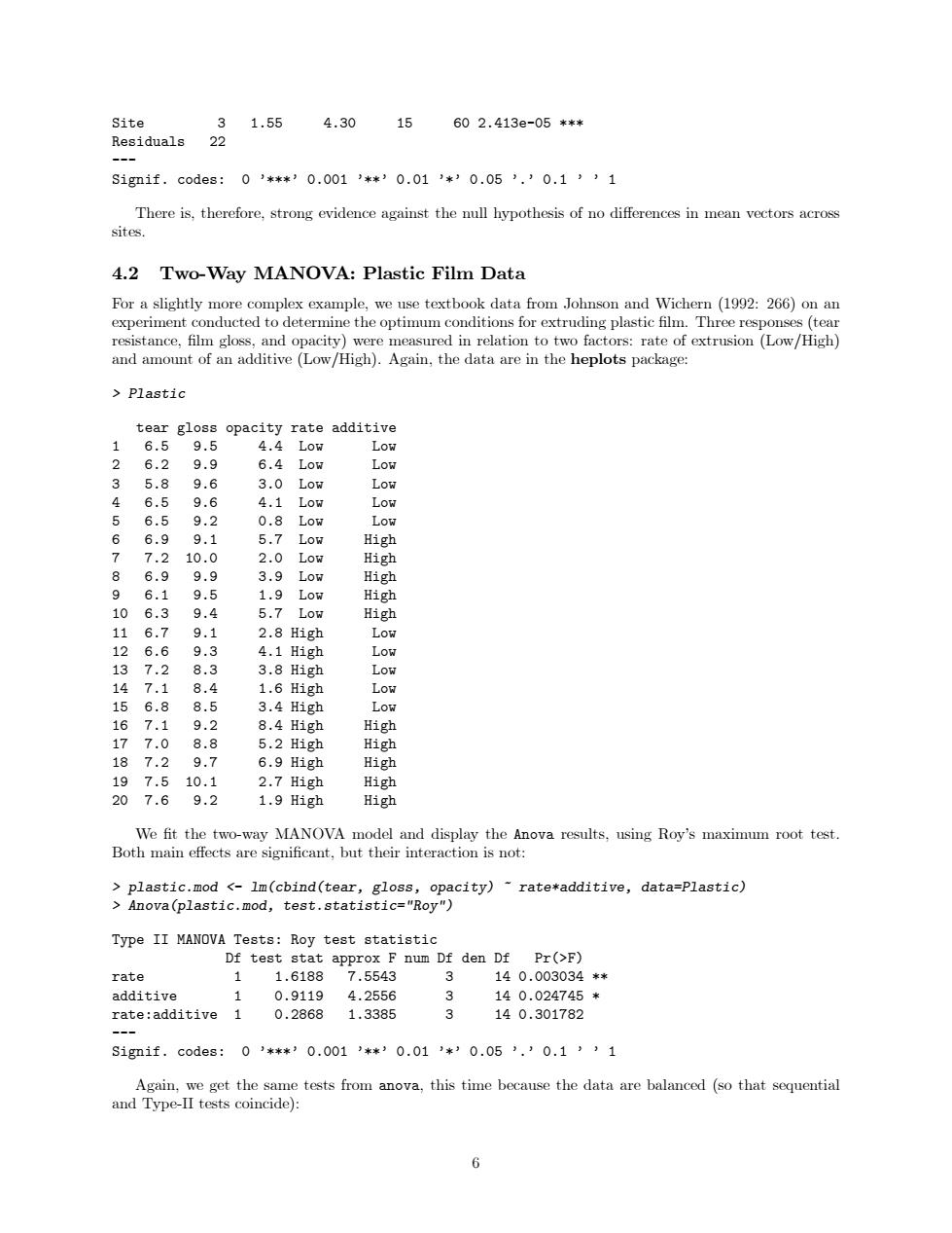
Site 31.55 4.30 15 602.413e-05*** Residuals 22 Signif.c0des:0J**’0.0013**’0.01’*’0.05’.’0.1’’1 There is,therefore,strong evidence against the null hypothesis of no differences in mean vectors across sites. 4.2 Two-Way MANOVA:Plastic Film Data For a slightly more complex example,we use textbook data from Johnson and Wichern (1992:266)on an experiment conducted to determine the optimum conditions for extruding plastic film.Three responses(tear resistance,film gloss,and opacity)were measured in relation to two factors:rate of extrusion (Low/High) and amount of an additive (Low/High).Again,the data are in the heplots package: Plastic tear gloss opacity rate additive 1 6.59.5 4.4 Low LoW 6.2 9.9 6.4 Low Low 3 5.8 9.6 3.0L0w LoW 4 6.5 9.6 4.1 Low LOW 6.5 9.2 0.8 Low LoW 6 6.9 9.1 5.7 Low High 7 7.2 10.0 2.0 Low High 6.9 9.9 3.9 Low Hig融 9 6.1 9.5 1.9 Low High 10 6.3 9.4 5.7 Low Hig助 11 6.7 9.1 2.8 High LOW 12 6.6 9.3 4.1 High LOW 13 7.2 8.3 3.8 High Low 14 7.1 8.4 1.6 High LOW 15 6.8 8.5 3.4 High LOw 16 7.1 9.2 8.4 High High 17 7.0 8.8 5.2 High High 18 7.2 9.7 6.9 High High 19 7.5 10.1 2.7 High High 20 7.6 9.2 1.9 High High We fit the two-way MANOVA model and display the Anova results,using Roy's maximum root test. Both main effects are significant,but their interaction is not: plastic.mod <-lm(cbind(tear,gloss,opacity)~rate*additive,data=Plastic) Anova(plastic.mod,test.statistic="Roy") Type II MANOVA Tests:Roy test statistic Df test stat approx F num Df den Df Pr(>F) rate 1 1.61887.5543 3 140.003034** additive 1 0.9119 4.2556 3 140.024745* rate:additive 1 0.28681.3385 3 140.301782 Sig题if.c0des:0’**?0.001’*30.01’*’0.05).’0.1’)1 Again,we get the same tests from anova,this time because the data are balanced (so that sequential and Type-II tests coincide): 6Site 3 1.55 4.30 15 60 2.413e-05 *** Residuals 22 --- Signif. codes: 0 ’***’ 0.001 ’**’ 0.01 ’*’ 0.05 ’.’ 0.1 ’ ’ 1 There is, therefore, strong evidence against the null hypothesis of no differences in mean vectors across sites. 4.2 Two-Way MANOVA: Plastic Film Data For a slightly more complex example, we use textbook data from Johnson and Wichern (1992: 266) on an experiment conducted to determine the optimum conditions for extruding plastic film. Three responses (tear resistance, film gloss, and opacity) were measured in relation to two factors: rate of extrusion (Low/High) and amount of an additive (Low/High). Again, the data are in the heplots package: > Plastic tear gloss opacity rate additive 1 6.5 9.5 4.4 Low Low 2 6.2 9.9 6.4 Low Low 3 5.8 9.6 3.0 Low Low 4 6.5 9.6 4.1 Low Low 5 6.5 9.2 0.8 Low Low 6 6.9 9.1 5.7 Low High 7 7.2 10.0 2.0 Low High 8 6.9 9.9 3.9 Low High 9 6.1 9.5 1.9 Low High 10 6.3 9.4 5.7 Low High 11 6.7 9.1 2.8 High Low 12 6.6 9.3 4.1 High Low 13 7.2 8.3 3.8 High Low 14 7.1 8.4 1.6 High Low 15 6.8 8.5 3.4 High Low 16 7.1 9.2 8.4 High High 17 7.0 8.8 5.2 High High 18 7.2 9.7 6.9 High High 19 7.5 10.1 2.7 High High 20 7.6 9.2 1.9 High High We fit the two-way MANOVA model and display the Anova results, using Roy’s maximum root test. Both main effects are significant, but their interaction is not: > plastic.mod <- lm(cbind(tear, gloss, opacity) ~ rate*additive, data=Plastic) > Anova(plastic.mod, test.statistic="Roy") Type II MANOVA Tests: Roy test statistic Df test stat approx F num Df den Df Pr(>F) rate 1 1.6188 7.5543 3 14 0.003034 ** additive 1 0.9119 4.2556 3 14 0.024745 * rate:additive 1 0.2868 1.3385 3 14 0.301782 --- Signif. codes: 0 ’***’ 0.001 ’**’ 0.01 ’*’ 0.05 ’.’ 0.1 ’ ’ 1 Again, we get the same tests from anova, this time because the data are balanced (so that sequential and Type-II tests coincide): 6