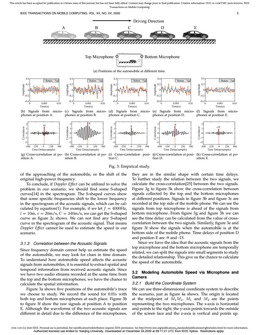
This article has been accepted for publication in a future issue of this journal,but has not been fully edited.Content may change prior to final publication.Citation information:DOI 10.1109/TMC.2020.3034354.IEEE Transactions on Mobile Computing IEEE TRANSACTIONS ON MOBILE COMPUTING,VOL.XX,NO.XX,2020 5 Driving Direction B D Top Microphone Bottom Microphone (a)Positions of the automobile at different time. 0. 04 -Bottom-Top Bottom-Top Bottom-Top Bottom-Top Bottom-Tc 13 A. -0 -03 -0 0.005 0.01 0.005 0.01 0.005 0.01 0.005 0.0 0.005 0.01 Time(s) Time(s) Time(s) Time(s) Time(s) (b)Signals from micro-(c)Signals from micro-(d)Signals from micro-(e)Signals from micro-(f)Signals from micro- phones at position A phones at position B. phones at position C. phones at position D. phones at position E. N-w 2 -2 -250 0 250 S0 500 -250 250 00 -250 0 250 00 -250 250 -500 -250 0 250 00 Time Delay(sample) Time Delay(sample) Time Delay(sample) Time Delay(sample) Time Delay(sample) (g)Cross-correlation at po-(h)Cross-correlation at po- (i)Cross-correlation posi- (j)Cross-correlation at posi-(k)Cross-correlation at po- sition A. sition B. tion C. tion D. sition E. Fig.3:Empirical study. of the approaching of the automobile,or the shift of the they are in the similar shape with certain time delays. original high-power frequency. To further study the relation between the two signals,we To conclude,if Doppler Effect can be utilized to solve the calculate the cross-correlation[25]between the two signals. problem in our scenario,we should find some S-shaped Figure 3g to figure 3k show the cross-correlation between curves[14]in the spectrogram.The S-shaped curves show signals collected by the top and the bottom microphones that some specific frequencies shift to the lower frequency at different positions.Signals in figure 3b and figure 3c are in the spectrogram of the acoustic signals,which can be cal- recorded at the top side of the mobile phone.We can see the culated by equation(1).For example,if we let f =4000Hz signals from top microphone is ahead of the signals from I 10m,v =20m/s,C=340m/s,we can get the S-shaped bottom microphone.From figure 3g and figure 3h we can curve as figure 2c shows.We can not find any S-shaped see the time delay can be calculated from the value of cross- curve in the spectrogram of the acoustic signal.That means correlation between the two signals.Similarly,figure 3e and Doppler Efect cannot be used to estimate the speed in our figure 3f show the signals when the automobile is at the scenario. bottom side of the mobile phone.Time delays of position D and position E are-9 and-15. 3.1.3 Correlation between the Acoustic Signals Since we have the idea that the acoustic signals from the Since frequency domain cannot help us estimate the speed top microphone and the bottom microphone are temporally of the automobile,we may look for clues in time domain. related,we can split the signals into small segments to study To understand how automobile speed affects the acoustic the detailed relationship.This give us the chance to calculate signals from automobiles,it is essential to extract spatial and the speed of the automobile. temporal information from received acoustic signals.Since we have two audio streams recorded at the same time from 3.2 Modeling Automobile Speed via Microphone and the top and the bottom microphones,we have the chance to Camera calculate the spatial information. 3.2.1 Build the Coordinate System Figure 3a shows five positions of the automobile's trace We can use three-dimensional coordinate system to describe we choose to study.We record the sound for 0.01s with the scenario,just as figure 4a shows.The origin is located both top and bottom microphones at each place.Figure 3b at the midpoint of MiM2.M and M2 are the points to figure 3f show the raw signals at position A to position representing the two microphones.The x-axis is horizontal E.Although the waveforms of the two acoustic signals are and points to the right,the y-axis points towards the outside different in detail due to the difference of the microphones, of the screen face and the z-axis is vertical and points up. 36-1233(c)2020 IEEE Personal use is permitted,but republication/redistribution requires IEEE permission.See http://www.ieee.org/publications_standards/publications/rights/index.html for more information. Authorized licensed use limited to:Nanjing University.Downloaded on December 24,2020 at 09:11:21 UTC from IEEE Xplore.Restrictions apply.1536-1233 (c) 2020 IEEE. Personal use is permitted, but republication/redistribution requires IEEE permission. See http://www.ieee.org/publications_standards/publications/rights/index.html for more information. This article has been accepted for publication in a future issue of this journal, but has not been fully edited. Content may change prior to final publication. Citation information: DOI 10.1109/TMC.2020.3034354, IEEE Transactions on Mobile Computing IEEE TRANSACTIONS ON MOBILE COMPUTING, VOL. XX, NO. XX, 2020 5 A B C D E Driving Direction Top Microphone Bottom Microphone (a) Positions of the automobile at different time. 0 0.005 0.01 Time(s) -0.4 -0.2 0 0.2 0.4 Amplitude Bottom Top (b) Signals from micro￾phones at position A. 0 0.005 0.01 Time(s) -0.4 -0.2 0 0.2 0.4 Amplitude Bottom Top (c) Signals from micro￾phones at position B. 0 0.005 0.01 Time(s) -0.4 -0.2 0 0.2 0.4 Amplitude Bottom Top (d) Signals from micro￾phones at position C. 0 0.005 0.01 Time(s) -0.4 -0.2 0 0.2 0.4 Amplitude Bottom Top (e) Signals from micro￾phones at position D. 0 0.005 0.01 Time(s) -0.4 -0.2 0 0.2 0.4 Amplitude Bottom Top (f) Signals from micro￾phones at position E. -500 -250 0 250 500 Time Delay(sample) -2 -1 0 1 2 Correlation 19 (g) Cross-correlation at po￾sition A. -500 -250 0 250 500 Time Delay(sample) -2 -1 0 1 2 Correlation 8 (h) Cross-correlation at po￾sition B. -500 -250 0 250 500 Time Delay(sample) -2 -1 0 1 2 Correlation 0 (i) Cross-correlation posi￾tion C. -500 -250 0 250 500 Time Delay(sample) -2 -1 0 1 2 Correlation -9 (j) Cross-correlation at posi￾tion D. -500 -250 0 250 500 Time Delay(sample) -2 -1 0 1 2 Correlation -15 (k) Cross-correlation at po￾sition E. Fig. 3: Empirical study. of the approaching of the automobile, or the shift of the original high-power frequency. To conclude, if Doppler Effect can be utilized to solve the problem in our scenario, we should find some S-shaped curves[14] in the spectrogram. The S-shaped curves show that some specific frequencies shift to the lower frequency in the spectrogram of the acoustic signals, which can be cal￾culated by equation(1). For example, if we let f = 4000Hz, l = 10m, v = 20m/s, C = 340m/s, we can get the S-shaped curve as figure 2c shows. We can not find any S-shaped curve in the spectrogram of the acoustic signal. That means Doppler Effect cannot be used to estimate the speed in our scenario. 3.1.3 Correlation between the Acoustic Signals Since frequency domain cannot help us estimate the speed of the automobile, we may look for clues in time domain. To understand how automobile speed affects the acoustic signals from automobiles, it is essential to extract spatial and temporal information from received acoustic signals. Since we have two audio streams recorded at the same time from the top and the bottom microphones, we have the chance to calculate the spatial information. Figure 3a shows five positions of the automobile’s trace we choose to study. We record the sound for 0.01s with both top and bottom microphones at each place. Figure 3b to figure 3f show the raw signals at position A to position E. Although the waveforms of the two acoustic signals are different in detail due to the difference of the microphones, they are in the similar shape with certain time delays. To further study the relation between the two signals, we calculate the cross-correlation[25] between the two signals. Figure 3g to figure 3k show the cross-correlation between signals collected by the top and the bottom microphones at different positions. Signals in figure 3b and figure 3c are recorded at the top side of the mobile phone. We can see the signals from top microphone is ahead of the signals from bottom microphone. From figure 3g and figure 3h we can see the time delay can be calculated from the value of cross￾correlation between the two signals. Similarly, figure 3e and figure 3f show the signals when the automobile is at the bottom side of the mobile phone. Time delays of position D and position E are -9 and -15. Since we have the idea that the acoustic signals from the top microphone and the bottom microphone are temporally related, we can split the signals into small segments to study the detailed relationship. This give us the chance to calculate the speed of the automobile. 3.2 Modeling Automobile Speed via Microphone and Camera 3.2.1 Build the Coordinate System We can use three-dimensional coordinate system to describe the scenario, just as figure 4a shows. The origin is located at the midpoint of M1M2. M1 and M2 are the points representing the two microphones. The x-axis is horizontal and points to the right, the y-axis points towards the outside of the screen face and the z-axis is vertical and points up. Authorized licensed use limited to: Nanjing University. Downloaded on December 24,2020 at 09:11:21 UTC from IEEE Xplore. Restrictions apply