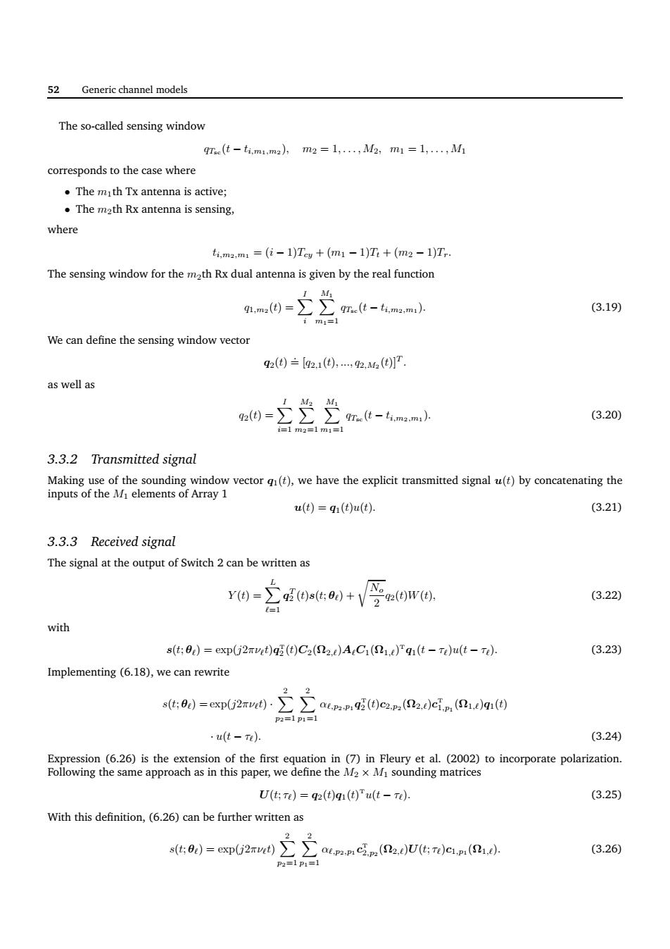
52 Generic channel models The so-called sensing window me(t-tm1.m,m2=1,,M,m1=1,M corresponds to the case where .The mth Tx antenna is active; The math Rx antenna is sensing. where t.mm=(-1Tg+(m-1T+(m2-1)T, The sensing window for the math Rx dual antenna is given by the real function q1.md-∑∑rt-t.m2m) (3.19 m= We can define the sensing window vector q2()=21(),2.2t)P. as well as 3.20) 3.3.2 Transmitted signal u()=q1(t)u(). (3.21) 3.3.3 Received signal The signal at the output of Switch 2 can be written as ((0w(. (3.22) with s(t:0c)=exp(j2vt)(t)C2()A.C(L)g(t-Te)u(t-Te). (3.23) Implementing(6.18),we can rewrite 8助=pU2-(o(ei(0 Pamlpim1 u(t-r). (3.24) li e ee the ne mm ension of the first equation in (7)in Fleury et al.(2002)to incorporate polarization. U(t:n)=q2(t)a(t)"u(t-r) (3.25) With this definition,(6.26)can be further written as (a.U(t:T)(S) (3.26) 52 Generic channel models The so-called sensing window qTsc (t − ti,m1,m2 ), m2 = 1, . . . , M2, m1 = 1, . . . , M1 corresponds to the case where • The m1th Tx antenna is active; • The m2th Rx antenna is sensing, where ti,m2,m1 = (i − 1)Tcy + (m1 − 1)Tt + (m2 − 1)Tr. The sensing window for the m2th Rx dual antenna is given by the real function q1,m2 (t) = X I i X M1 m1=1 qTsc (t − ti,m2,m1 ). (3.19) We can define the sensing window vector q2(t) .= [q2,1(t), ..., q2,M2 (t)]T . as well as q2(t) = X I i=1 X M2 m2=1 X M1 m1=1 qTsc (t − ti,m2,m1 ). (3.20) 3.3.2 Transmitted signal Making use of the sounding window vector q1(t), we have the explicit transmitted signal u(t) by concatenating the inputs of the M1 elements of Array 1 u(t) = q1(t)u(t). (3.21) 3.3.3 Received signal The signal at the output of Switch 2 can be written as Y (t) = X L ℓ=1 q T 2 (t)s(t; θℓ) + r No 2 q2(t)W(t), (3.22) with s(t; θℓ) = exp(j2πνℓt)q T 2 (t)C2(Ω2,ℓ)AℓC1(Ω1,ℓ) T q1(t − τℓ)u(t − τℓ). (3.23) Implementing (6.18), we can rewrite s(t; θℓ) = exp(j2πνℓt) · X 2 p2=1 X 2 p1=1 αℓ,p2,p1 q T 2 (t)c2,p2 (Ω2,ℓ)c T 1,p1 (Ω1,ℓ)q1(t) · u(t − τℓ). (3.24) Expression (6.26) is the extension of the first equation in (7) in Fleury et al. (2002) to incorporate polarization. Following the same approach as in this paper, we define the M2 × M1 sounding matrices U(t; τℓ) = q2(t)q1(t) Tu(t − τℓ). (3.25) With this definition, (6.26) can be further written as s(t; θℓ) = exp(j2πνℓt) X 2 p2=1 X 2 p1=1 αℓ,p2,p1 c T 2,p2 (Ω2,ℓ)U(t; τℓ)c1,p1 (Ω1,ℓ). (3.26)