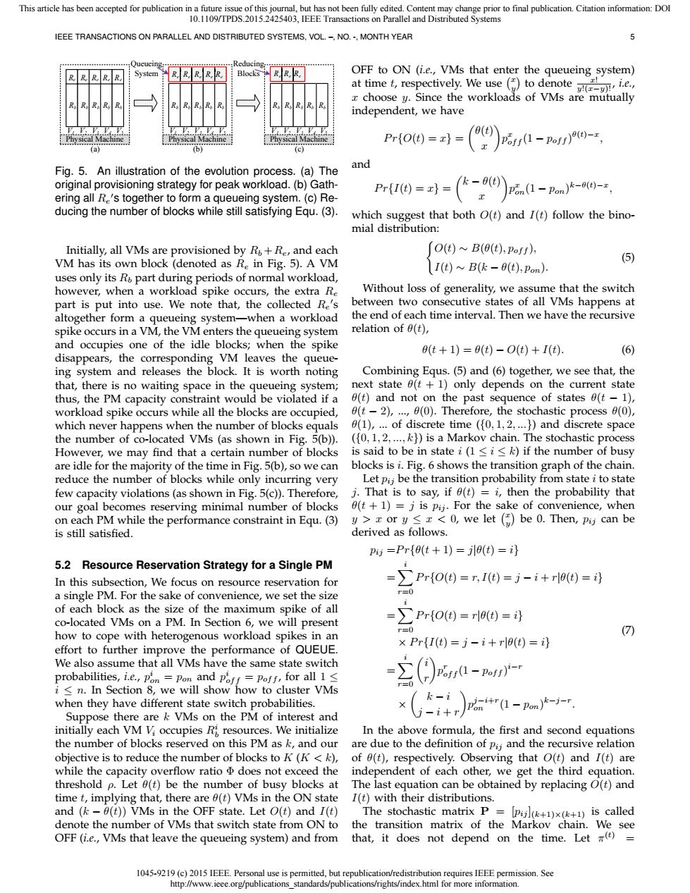
This article has been accepted for publication in a future issue of this journal,but has not been fully edited.Content may change prior to final publication.Citation information:DOI 10.1109/TPDS.2015.2425403,IEEE Transactions on Parallel and Distributed Systems IEEE TRANSACTIONS ON PARALLEL AND DISTRIBUTED SYSTEMS,VOL.-.NO.-,MONTH YEAR Queueing: Reducing R RR RR System Blocks OFF to ON (i.e.,VMs that enter the queueing system) at timet,respectively.We use (to denoteie x choose y.Since the workloads of VMs are mutually independent,we have Physical Machine cal Machine Physical Machine Pr{O(t)=x}= ）P1-pof)- @(t) (a) (b) (c) and Fig.5.An illustration of the evolution process.(a)The original provisioning strategy for peak workload.(b)Gath- Pr{I(t)=x}= ering all R's together to form a queueing system.(c)Re- k-e）p6n(1-pom-- ducing the number of blocks while still satisfying Equ.(3). which suggest that both O(t)and I(t)follow the bino- mial distribution: Initially,all VMs are provisioned by R+Re,and each O(t)B(0(t),Poff), VM has its own block (denoted as Re in Fig.5).A VM (5) I(t)~B(k-0(t);Pon). uses only its Ro part during periods of normal workload, however,when a workload spike occurs,the extra Re Without loss of generality,we assume that the switch part is put into use.We note that,the collected Re's between two consecutive states of all VMs happens at altogether form a queueing system-when a workload the end of each time interval.Then we have the recursive spike occurs in a VM,the VM enters the queueing system relation of (t), and occupies one of the idle blocks;when the spike (t+1)=θ(t)-O(t)+I(t) (6) disappears,the corresponding VM leaves the queue- ing system and releases the block.It is worth noting Combining Equs.(5)and(6)together,we see that,the that,there is no waiting space in the queueing system; next state (t+1)only depends on the current state thus,the PM capacity constraint would be violated if a 0(t)and not on the past sequence of states 0(t-1), workload spike occurs while all the blocks are occupied,(t-2),...,0(0).Therefore,the stochastic process (0), which never happens when the number of blocks equals 0(1),...of discrete time (10,1,2,...})and discrete space the number of co-located VMs (as shown in Fig.5(b)). ([0,1,2,...,))is a Markov chain.The stochastic process However,we may find that a certain number of blocks is said to be in state i(1<i<k)if the number of busy are idle for the majority of the time in Fig.5(b),so we can blocks is i.Fig.6 shows the transition graph of the chain. reduce the number of blocks while only incurring very Let pij be the transition probability from state i to state few capacity violations(as shown in Fig.5(c)).Therefore,j.That is to say,if (t)=i,then the probability that our goal becomes reserving minimal number of blocks 0(t+1)=j is pij.For the sake of convenience,when on each PM while the performance constraint in Equ.(3) y>x or y<x<0,we let (be 0.Then,Pij can be is still satisfied. derived as follows. p=Pr{9(t+1)=(t)= 5.2 Resource Reservation Strategy for a Single PM In this subsection,We focus on resource reservation for =∑Pr0=因=j-i+r8= a single PM.For the sake of convenience,we set the size r=0 of each block as the size of the maximum spike of all co-located VMs on a PM.In Section 6,we will present =∑Pr{O(=r(=i r=0 how to cope with heterogenous workload spikes in an (7) effort to further improve the performance of QUEUE. x Pr{I(t)=j-i+0(t)=i} We also assume that all VMs have the same state switch probabilities,i.e.,pon =Pon and poff=Poff,for all 1< i<n.In Section 8,we will show how to cluster VMs when they have different state switch probabilities. Suppose there are k VMs on the PM of interest and initially each VM Vi occupies R resources.We initialize In the above formula,the first and second equations the number of blocks reserved on this PM as k,and our are due to the definition of pij and the recursive relation objective is to reduce the number of blocks to K(K<k), of 0(t),respectively.Observing that O(t)and I(t)are while the capacity overflow ratio does not exceed the independent of each other,we get the third equation threshold p.Let 0(t)be the number of busy blocks at The last equation can be obtained by replacing O(t)and time t,implying that,there are 0(t)VMs in the ON state I(t)with their distributions. and (k-0(t))VMs in the OFF state.Let O(t)and I(t)The stochastic matrix P=pijl(+)x(+)is called denote the number of VMs that switch state from ON to the transition matrix of the Markov chain.We see OFF(i.e.,VMs that leave the queueing system)and from that,it does not depend on the time.Let () 1045-9219(c)2015 IEEE.Personal use is permitted,but republication/redistribution requires IEEE permission.See http://www.ieee.org/publications standards/publications/rights/index.html for more information.1045-9219 (c) 2015 IEEE. Personal use is permitted, but republication/redistribution requires IEEE permission. See http://www.ieee.org/publications_standards/publications/rights/index.html for more information. This article has been accepted for publication in a future issue of this journal, but has not been fully edited. Content may change prior to final publication. Citation information: DOI 10.1109/TPDS.2015.2425403, IEEE Transactions on Parallel and Distributed Systems IEEE TRANSACTIONS ON PARALLEL AND DISTRIBUTED SYSTEMS, VOL. –, NO. -, MONTH YEAR 5 Queueing System Physical Machine V1 V2 V3 V4 V5 Physical Machine Re Re Re Re Re Reducing Blocks Physical Machine Re Re Re (a) (b) (c) Re Re Re Re Re V1 V2 V3 V4 V5 V1 V2 V3 V4 V5 Rb Rb Rb Rb Rb Rb Rb Rb Rb Rb Rb Rb Rb Rb Rb Fig. 5. An illustration of the evolution process. (a) The original provisioning strategy for peak workload. (b) Gath￾ering all Re ′s together to form a queueing system. (c) Re￾ducing the number of blocks while still satisfying Equ. (3). Initially, all VMs are provisioned by Rb +Re, and each VM has its own block (denoted as Re in Fig. 5). A VM uses only its Rb part during periods of normal workload, however, when a workload spike occurs, the extra Re part is put into use. We note that, the collected Re ′ s altogether form a queueing system—when a workload spike occurs in a VM, the VM enters the queueing system and occupies one of the idle blocks; when the spike disappears, the corresponding VM leaves the queue￾ing system and releases the block. It is worth noting that, there is no waiting space in the queueing system; thus, the PM capacity constraint would be violated if a workload spike occurs while all the blocks are occupied, which never happens when the number of blocks equals the number of co-located VMs (as shown in Fig. 5(b)). However, we may find that a certain number of blocks are idle for the majority of the time in Fig. 5(b), so we can reduce the number of blocks while only incurring very few capacity violations (as shown in Fig. 5(c)). Therefore, our goal becomes reserving minimal number of blocks on each PM while the performance constraint in Equ. (3) is still satisfied. 5.2 Resource Reservation Strategy for a Single PM In this subsection, We focus on resource reservation for a single PM. For the sake of convenience, we set the size of each block as the size of the maximum spike of all co-located VMs on a PM. In Section 6, we will present how to cope with heterogenous workload spikes in an effort to further improve the performance of QUEUE. We also assume that all VMs have the same state switch probabilities, i.e., p i on = pon and p i of f = poff , for all 1 ≤ i ≤ n. In Section 8, we will show how to cluster VMs when they have different state switch probabilities. Suppose there are k VMs on the PM of interest and initially each VM Vi occupies Ri b resources. We initialize the number of blocks reserved on this PM as k, and our objective is to reduce the number of blocks to K (K < k), while the capacity overflow ratio Φ does not exceed the threshold ρ. Let θ(t) be the number of busy blocks at time t, implying that, there are θ(t) VMs in the ON state and (k − θ(t)) VMs in the OFF state. Let O(t) and I(t) denote the number of VMs that switch state from ON to OFF (i.e., VMs that leave the queueing system) and from OFF to ON (i.e., VMs that enter the queueing system) at time t, respectively. We use ( x y ) to denote x! y!(x−y)! , i.e., x choose y. Since the workloads of VMs are mutually independent, we have P r{O(t) = x} = ( θ(t) x ) p x of f (1 − poff ) θ(t)−x , and P r{I(t) = x} = ( k − θ(t) x ) p x on(1 − pon) k−θ(t)−x , which suggest that both O(t) and I(t) follow the bino￾mial distribution: { O(t) ∼ B(θ(t), poff ), I(t) ∼ B(k − θ(t), pon). (5) Without loss of generality, we assume that the switch between two consecutive states of all VMs happens at the end of each time interval. Then we have the recursive relation of θ(t), θ(t + 1) = θ(t) − O(t) + I(t). (6) Combining Equs. (5) and (6) together, we see that, the next state θ(t + 1) only depends on the current state θ(t) and not on the past sequence of states θ(t − 1), θ(t − 2), ..., θ(0). Therefore, the stochastic process θ(0), θ(1), ... of discrete time ({0, 1, 2, ...}) and discrete space ({0, 1, 2, ..., k}) is a Markov chain. The stochastic process is said to be in state i (1 ≤ i ≤ k) if the number of busy blocks is i. Fig. 6 shows the transition graph of the chain. Let pij be the transition probability from state i to state j. That is to say, if θ(t) = i, then the probability that θ(t + 1) = j is pij . For the sake of convenience, when y > x or y ≤ x < 0, we let ( x y ) be 0. Then, pij can be derived as follows. pij =P r{θ(t + 1) = j|θ(t) = i} = ∑ i r=0 P r{O(t) = r, I(t) = j − i + r|θ(t) = i} = ∑ i r=0 P r{O(t) = r|θ(t) = i} × P r{I(t) = j − i + r|θ(t) = i} = ∑ i r=0 ( i r ) p r off (1 − poff ) i−r × ( k − i j − i + r ) p j−i+r on (1 − pon) k−j−r . (7) In the above formula, the first and second equations are due to the definition of pij and the recursive relation of θ(t), respectively. Observing that O(t) and I(t) are independent of each other, we get the third equation. The last equation can be obtained by replacing O(t) and I(t) with their distributions. The stochastic matrix P = [pij ](k+1)×(k+1) is called the transition matrix of the Markov chain. We see that, it does not depend on the time. Let π (t) =