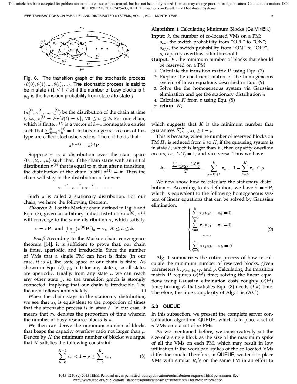
This article has been accepted for publication in a future issue of this journal,but has not been fully edited.Content may change prior to final publication.Citation information:DOI 10.1109/TPDS.2015.2425403,IEEE Transactions on Parallel and Distributed Systems IEEE TRANSACTIONS ON PARALLEL AND DISTRIBUTED SYSTEMS,VOL.-.NO.-,MONTH YEAR 6 Algorithm 1 Calculating Minimum Blocks(CalMinBlk) Input:k,the number of co-located VMs on a PM; Pon,the switch probability from "OFF"to "ON"; Poff,the switch probability from "ON"to "OFF"; P,capacity overflow ratio threshold Output:K,the minimum number of blocks that should be reserved on a PM 1:Calculate the transition matrix P using Equ.(7) Fig.6.The transition graph of the stochastic process 2:Prepare the coefficient matrix of the homogeneous {(0),(1),...,0(t),....The stochastic process is said to system of linear equations described in Equ.(9) be in state i(1<i<k)if the number of busy blocks is i. 3:Solve the the homogeneous system via Gaussian pj is the transition probability from state i to state j. elimination and get the stationary distribution m 4: Calculate K from m using Equ.(8) ()be the distribution of the chain at time 5:return K; t,ie,T9=Pr{a(t)=n,0≤h≤k.For our chain, which is finite,()is a vector ofk+1 nonnegative entries which suggests that K is the minimum number that such that1.In linear algebra,vectors of this guarantees∑KoTn≥1-p type are called stochastic vectors.Then,it holds that This is because,when he number of reserved blocks on π(t+1)=π()P PM Hi is reduced from k to K,if the queueing system is in state h,which is larger than K,then capacity overflow Suppose is a distribution over the state space occurs,i.e.,CO!=1,and vice versa.Thus we have (0,1,2,...,k}such that,if the chain starts with an initial K distribution (0)that is equal to m,then after a transition, the distribution of the chain is still (1)=T.Then the T 元=1-∑h≤P h=K+1 h=0 chain will stay in the distribution m forever: We now show how to calculate the stationary distri- 开PπPπP bution m.According to its definition,we have =P, Such is called a stationary distribution.For our which is equivalent to the following homogeneous sys- chain,we have the following theorem. tem of linear equations that can be solved by Gaussian Theorem 2:For the Markov chain defined in Fig.6 and elimination Equ.(7),given an arbitrary initial distribution (),( ThPho -T0 =0 will converge to the same distribution m,which satisify π=πP,and lim(πoPt)h=Th,0≤h≤k. hPh1-π1=0 (9) →o Proof:According to the Markov chain convergence theorem [14],it is sufficient to prove that,our chain is finite,aperiodic,and irreducible.Since the number ThPhk -TTk =0 h=k of VMs that a single PM can host is finite (in our Alg.1 summarizes the entire process of how to cal- case,it is k),the state space of our chain is finite.As culate the minimum number of reserved blocks,given shown in Equ.(7),pi >0 for any state i,so all states parameters k,Pon,Poff,and p.Calculating the transition are aperiodic.Finally,from any state i,we can reach matrix P requires O(k3)time;solving the linear equa- any other state j,so the transition graph is strongly tions using Gaussian elimination costs roughly O(k3) connected,implying that our chain is irreducible.The time;finding K that satisfies Equ.(8)needs O(k)time. theorem follows immediately. Therefore,the time complexity of Alg.1 is O(k3). When the chain stays in the stationary distribution, we see that Th is equivalent to the proportion of times that the stochastic process is in state h.In our case,it 5.3 QUEUE means that mh denotes the proportion of time wherein In this subsection,we present the complete server con- the number of busy resource blocks is h. solidation algorithm,QUEUE,which is to place a set of We then can derive the minimum number of blocks n VMs onto a set of m PMs. that keeps the capacity overflow ratio not larger than p. As we mentioned before,we conservatively set the Denote by K the minimum number of blocks;we argue size of a single block as the size of the maximum spike that K satisfies the following constraint: of all the VMs on each PM,which may result in low K-1 K utilization if the workload spikes of the co-located VMs Th<1-p≤ (8) differ too much.Therefore,in QUEUE,we tend to place h-0 h=0 VMs with similar Re's on the same PM in an effort to 1045-9219(c)2015 IEEE.Personal use is permitted,but republication/redistribution requires IEEE permission.See http://www.ieee.org/publications standards/publications/rights/index.html for more information.1045-9219 (c) 2015 IEEE. Personal use is permitted, but republication/redistribution requires IEEE permission. See http://www.ieee.org/publications_standards/publications/rights/index.html for more information. This article has been accepted for publication in a future issue of this journal, but has not been fully edited. Content may change prior to final publication. Citation information: DOI 10.1109/TPDS.2015.2425403, IEEE Transactions on Parallel and Distributed Systems IEEE TRANSACTIONS ON PARALLEL AND DISTRIBUTED SYSTEMS, VOL. –, NO. -, MONTH YEAR 6 p00 0 1 2 k p0k p02 p01 p12 p1k p10 p11 p2k p22 p21 p20 pk0 pk1 pk2 pkk Fig. 6. The transition graph of the stochastic process {θ(0), θ(1), ..., θ(t), ...}. The stochastic process is said to be in state i (1 ≤ i ≤ k) if the number of busy blocks is i. pij is the transition probability from state i to state j. (π (t) 0 , π (t) 1 , ..., π (t) k ) be the distribution of the chain at time t, i.e., π (t) h = P r{θ(t) = h}, ∀0 ≤ h ≤ k. For our chain, which is finite, π (t) is a vector of k+1 nonnegative entries such that ∑k h=0 π (t) h = 1. In linear algebra, vectors of this type are called stochastic vectors. Then, it holds that π (t+1) = π (t)P. Suppose π is a distribution over the state space {0, 1, 2, ..., k} such that, if the chain starts with an initial distribution π (0) that is equal to π, then after a transition, the distribution of the chain is still π (1) = π. Then the chain will stay in the distribution π forever: π P −→ π P −→ π P −→ · · · · · · Such π is called a stationary distribution. For our chain, we have the following theorem. Theorem 2: For the Markov chain defined in Fig. 6 and Equ. (7), given an arbitrary initial distribution π (0) , π (t) will converge to the same distribution π, which satisify π = πP, and limt→∞ (π (0)P t )h = πh, ∀0 ≤ h ≤ k. Proof: According to the Markov chain convergence theorem [14], it is sufficient to prove that, our chain is finite, aperiodic, and irreducible. Since the number of VMs that a single PM can host is finite (in our case, it is k), the state space of our chain is finite. As shown in Equ. (7), pii > 0 for any state i, so all states are aperiodic. Finally, from any state i, we can reach any other state j, so the transition graph is strongly connected, implying that our chain is irreducible. The theorem follows immediately. When the chain stays in the stationary distribution, we see that πh is equivalent to the proportion of times that the stochastic process is in state h. In our case, it means that πh denotes the proportion of time wherein the number of busy resource blocks is h. We then can derive the minimum number of blocks that keeps the capacity overflow ratio not larger than ρ. Denote by K the minimum number of blocks; we argue that K satisfies the following constraint: K ∑−1 h=0 πh < 1 − ρ ≤ ∑ K h=0 πh, (8) Algorithm 1 Calculating Minimum Blocks (CalMinBlk) Input: k, the number of co-located VMs on a PM; pon, the switch probability from “OFF” to “ON”; pof f , the switch probability from “ON” to “OFF”; ρ, capacity overflow ratio threshold Output: K, the minimum number of blocks that should be reserved on a PM 1: Calculate the transition matrix P using Equ. (7) 2: Prepare the coefficient matrix of the homogeneous system of linear equations described in Equ. (9) 3: Solve the the homogeneous system via Gaussian elimination and get the stationary distribution π 4: Calculate K from π using Equ. (8) 5: return K; which suggests that K is the minimum number that guarantees ∑K h=0 πh ≥ 1 − ρ. This is because, when he number of reserved blocks on PM Hj is reduced from k to K, if the queueing system is in state h, which is larger than K, then capacity overflow occurs, i.e., COt j = 1, and vice versa. Thus we have Φj = ∑ 1≤t≤T COt j T = ∑ k h=K+1 πh = 1 − ∑ K h=0 πh ≤ ρ. We now show how to calculate the stationary distri￾bution π. According to its definition, we have π = πP, which is equivalent to the following homogeneous sys￾tem of linear equations that can be solved by Gaussian elimination.    ∑ k h=0 πhph0 − π0 = 0 ∑ k h=1 πhph1 − π1 = 0 ...... ∑ k h=k πhphk − πk = 0 (9) Alg. 1 summarizes the entire process of how to cal￾culate the minimum number of reserved blocks, given parameters k, pon, pof f , and ρ. Calculating the transition matrix P requires O(k 3 ) time; solving the linear equa￾tions using Gaussian elimination costs roughly O(k 3 ) time; finding K that satisfies Equ. (8) needs O(k) time. Therefore, the time complexity of Alg. 1 is O(k 3 ). 5.3 QUEUE In this subsection, we present the complete server con￾solidation algorithm, QUEUE, which is to place a set of n VMs onto a set of m PMs. As we mentioned before, we conservatively set the size of a single block as the size of the maximum spike of all the VMs on each PM, which may result in low utilization if the workload spikes of the co-located VMs differ too much. Therefore, in QUEUE, we tend to place VMs with similar Re ′ s on the same PM in an effort to