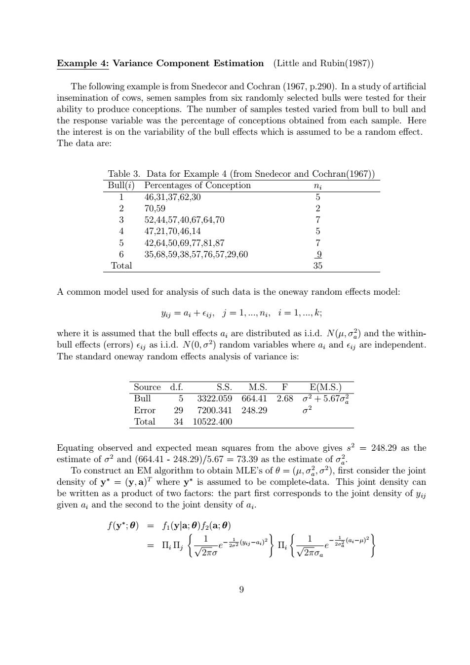
Example 4:Variance Component Estimation (Little and Rubin(1987)) The following example is from Snedecor and Cochran(1967,p.290).In a study of artificial insemination of cows,semen samples from six randomly selected bulls were tested for their ability to produce conceptions.The number of samples tested varied from bull to bull and the response variable was the percentage of conceptions obtained from each sample.Here the interest is on the variability of the bull effects which is assumed to be a random effect. The data are: Table 3.Data for Example 4 (from Snedecor and Cochran(1967)) Bull(i)Percentages of Conception ni 1 46,31,37.62,30 2 70.59 2 52,44,57,40,67,64,70 > 4 47,21,70,46,14 5 5 42,64,50,69,77,81,87 7 6 35,68,59,38,57,76,57,29,60 9 Total 35 A common model used for analysis of such data is the oneway random effects model: yij ai+eij,j=1,...,ni;i=1,...,k; where it is assumed that the bull effects ai are distributed as i.i.d.N(,o2)and the within- bull effects (errors)eij as i.i.d.N(0,o2)random variables where ai and ej are independent. The standard oneway random effects analysis of variance is: Source d.f. S.S. M.S. F E(M.S.) Bull 5 3322.059664.412.682+5.67o Error 29 7200.341248.29 02 Total 3410522.400 Equating observed and expected mean squares from the above gives s2=248.29 as the estimate of o2 and(664.41-248.29)/5.67 =73.39 as the estimate of o2 To construct an EM algorithm to obtain MLE's of =(u,o2,o2),first consider the joint density of y*=(y,a)T where y*is assumed to be complete-data.This joint density can be written as a product of two factors:the part first corresponds to the joint density of yij given ai and the second to the joint density of ai. f(y*;8)=fi(yla;0)f2(a;0) 9Example 4: Variance Component Estimation (Little and Rubin(1987)) The following example is from Snedecor and Cochran (1967, p.290). In a study of artificial insemination of cows, semen samples from six randomly selected bulls were tested for their ability to produce conceptions. The number of samples tested varied from bull to bull and the response variable was the percentage of conceptions obtained from each sample. Here the interest is on the variability of the bull effects which is assumed to be a random effect. The data are: Table 3. Data for Example 4 (from Snedecor and Cochran(1967)) Bull(i) Percentages of Conception ni 1 46,31,37,62,30 5 2 70,59 2 3 52,44,57,40,67,64,70 7 4 47,21,70,46,14 5 5 42,64,50,69,77,81,87 7 6 35,68,59,38,57,76,57,29,60 9 Total 35 A common model used for analysis of such data is the oneway random effects model: yij = ai + ij , j = 1, ..., ni , i = 1, ..., k; where it is assumed that the bull effects ai are distributed as i.i.d. N(µ, σ 2 a ) and the within￾bull effects (errors) ij as i.i.d. N(0, σ 2 ) random variables where ai and ij are independent. The standard oneway random effects analysis of variance is: Source d.f. S.S. M.S. F E(M.S.) Bull 5 3322.059 664.41 2.68 σ 2 + 5.67σ 2 a Error 29 7200.341 248.29 σ 2 Total 34 10522.400 Equating observed and expected mean squares from the above gives s 2 = 248.29 as the estimate of σ 2 and (664.41 - 248.29)/5.67 = 73.39 as the estimate of σ 2 a . To construct an EM algorithm to obtain MLE’s of θ = (µ, σ 2 a , σ 2 ), first consider the joint density of y ∗ = (y, a) T where y ∗ is assumed to be complete-data. This joint density can be written as a product of two factors: the part first corresponds to the joint density of yij given ai and the second to the joint density of ai . f(y ∗ ; θ) = f1(y|a; θ)f2(a; θ) = Πi Πj ( 1 √ 2πσ e − 1 2σ2 (yij−ai) 2 ) Πi ( 1 √ 2πσa e − 1 2σ2 a (ai−µ) 2 ) 9