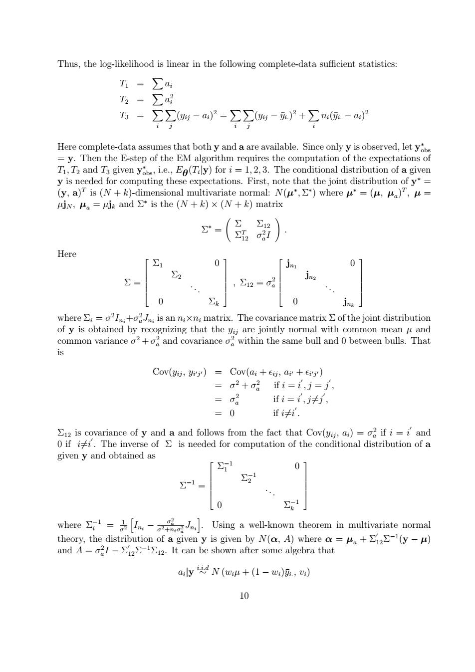
Thus,the log-likelihood is linear in the following complete-data sufficient statistics: T1= ∑a T2= ∑ =∑∑(-a)2=∑∑-.)2+∑n(.-a2 21 2.7 Here complete-data assumes that both y and a are available.Since only y is observed,let yo =y.Then the E-step of the EM algorithm requires the computation of the expectations of T1,T2 and T3 given yobs,i.e.,E(Tily)for i=1,2,3.The conditional distribution of a given y is needed for computing these expectations.First,note that the joint distribution of y*= (y,a)is (N+k)-dimensional multivariate normal:N(u*,>*)where u*=(u,u),u= jw,u。=jk and*is the(N+k)×(N+)matrix Here 1 07 ∑2 ∑= 12=2 0 ∑k」 0 jnk where i=o2In+02Jn is an nixni matrix.The covariance matrix of the joint distribution of y is obtained by recognizing that the yi;are jointly normal with common mean u and common variance o2+o2 and covariance o2 within the same bull and 0 between bulls.That is Cov(yij,yij)=Cov(ai+eij,ai+eij) = a2+0a ifi=i,j=j, =2 ifi=t,j≠j, =0 fi≠i. 12 is covariance of y and a and follows from the fact that Cov(yij,ai)=o2 if i=i and 0 if izi.The inverse of is needed for computation of the conditional distribution of a given y and obtained as 0 Σ1 21 0 where Using a well-known theorem in multivariate normal theory,the distribution of a given y is given by N(a,A)where a=ua+12(y-u) and A=2I-212.It can be shown after some algebra that a,lyN(wμ+(1-u),) 10Thus, the log-likelihood is linear in the following complete-data sufficient statistics: T1 = Xai T2 = Xa 2 i T3 = X i X j (yij − ai) 2 = X i X j (yij − y¯i.) 2 + X i ni(y¯i. − ai) 2 Here complete-data assumes that both y and a are available. Since only y is observed, let y ∗ obs = y. Then the E-step of the EM algorithm requires the computation of the expectations of T1, T2 and T3 given y ∗ obs, i.e., Eθ (Ti |y) for i = 1, 2, 3. The conditional distribution of a given y is needed for computing these expectations. First, note that the joint distribution of y ∗ = (y, a) T is (N + k)-dimensional multivariate normal: N(µ ∗ , Σ ∗ ) where µ ∗ = (µ, µa ) T , µ = µjN , µa = µjk and Σ ∗ is the (N + k) × (N + k) matrix Σ ∗ = Σ Σ12 Σ T 12 σ 2 a I ! . Here Σ =       Σ1 0 Σ2 . . . 0 Σk       , Σ12 = σ 2 a       jn1 0 jn2 . . . 0 jnk       where Σi = σ 2 Ini+σ 2 aJni is an ni×ni matrix. The covariance matrix Σ of the joint distribution of y is obtained by recognizing that the yij are jointly normal with common mean µ and common variance σ 2 + σ 2 a and covariance σ 2 a within the same bull and 0 between bulls. That is Cov(yij , yi 0j 0) = Cov(ai + ij , ai 0 + i 0j 0) = σ 2 + σ 2 a if i = i 0 , j = j 0 , = σ 2 a if i = i 0 , j6=j 0 , = 0 if i6=i 0 . Σ12 is covariance of y and a and follows from the fact that Cov(yij , ai) = σ 2 a if i = i 0 and 0 if i6=i 0 . The inverse of Σ is needed for computation of the conditional distribution of a given y and obtained as Σ −1 =       Σ −1 1 0 Σ −1 2 . . . 0 Σ −1 k       where Σ −1 i = 1 σ2 h Ini − σ 2 a σ2+niσ2 a Jni i . Using a well-known theorem in multivariate normal theory, the distribution of a given y is given by N(α, A) where α = µa + Σ 0 12Σ −1 (y − µ) and A = σ 2 a I − Σ 0 12Σ −1Σ12. It can be shown after some algebra that ai |y i.i.d ∼ N (wiµ + (1 − wi)y¯i., vi) 10