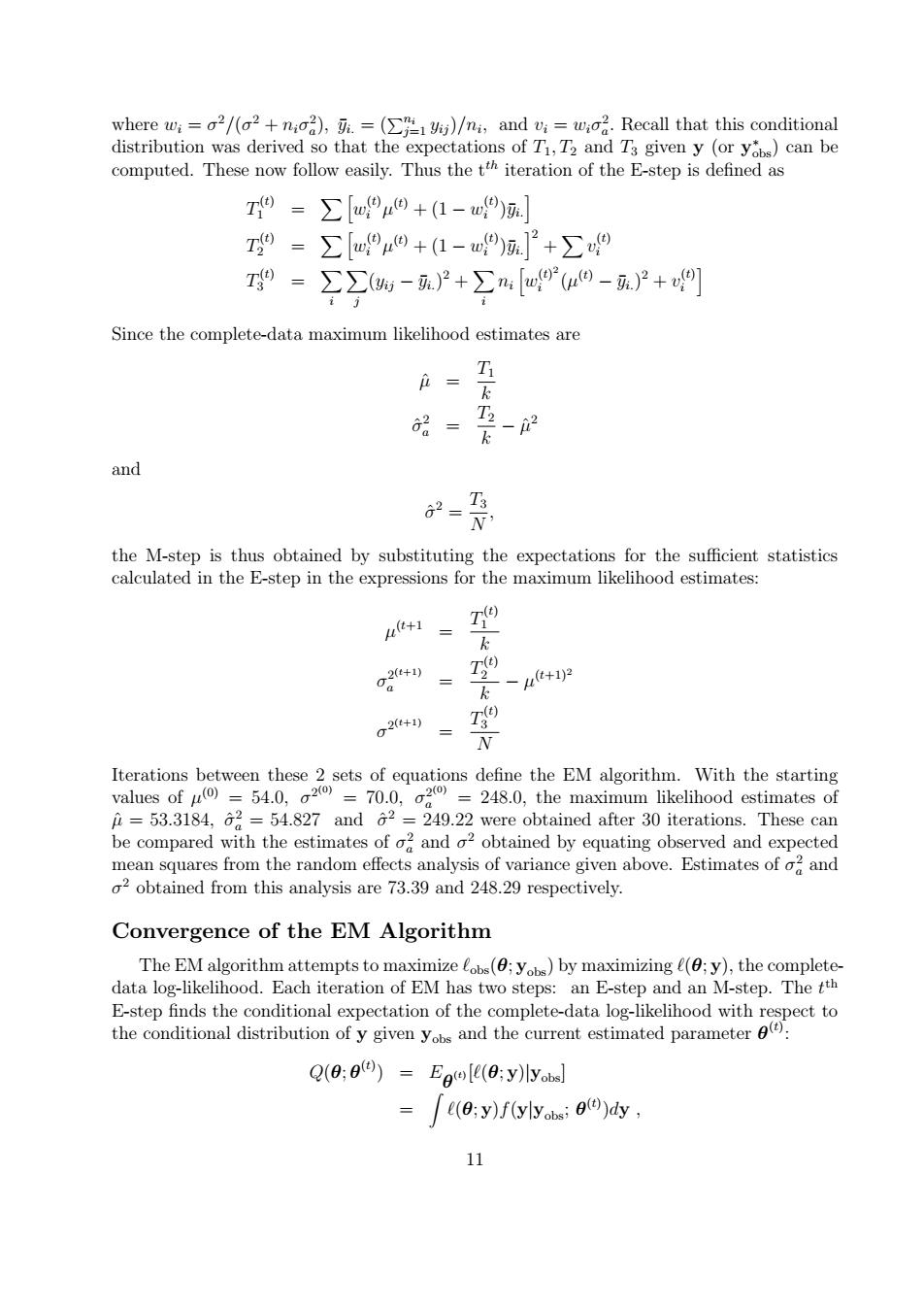
where wi=a2/(2+na),.=()/ni,and vi=w:oa.Recall that this conditional distribution was derived so that the expectations of T1,T2 and T3 given y (or yobs)can be computed.These now follow easily.Thus the tth iteration of the E-step is defined as 0=∑m9μ0+(1-w9) 79-∑9+1-w]+∑9 T9=∑∑(%-.)P+∑nm(9-2+9] Since the complete-data maximum likelihood estimates are = T 品= 2-2 and T the M-step is thus obtained by substituting the expectations for the sufficient statistics calculated in the E-step in the expressions for the maximum likelihood estimates: u+1= k 02 T k ~u+1)2 g2+1) N Iterations between these 2 sets of equations define the EM algorithm.With the starting values of ()=54.0,2)=70.0,2)=248.0,the maximum likelihood estimates of =53.3184,62 =54.827 and 62=249.22 were obtained after 30 iterations.These can be compared with the estimates of o2 and o2 obtained by equating observed and expected mean squares from the random effects analysis of variance given above.Estimates of o and o2 obtained from this analysis are 73.39 and 248.29 respectively. Convergence of the EM Algorithm The EM algorithm attempts to maximize lobs(6;yobs)by maximizing l(0;y),the complete- data log-likelihood.Each iteration of EM has two steps:an E-step and an M-step.The tth E-step finds the conditional expectation of the complete-data log-likelihood with respect to the conditional distribution of y given yos and the current estimated parameter) Q(0:0()=Egle(0;y)lyob = (0:y)f(ylyobdy, 11where wi = σ 2/(σ 2 + niσ 2 a ), y¯i. = ( Pni j=1 yij )/ni , and vi = wiσ 2 a . Recall that this conditional distribution was derived so that the expectations of T1, T2 and T3 given y (or y ∗ obs) can be computed. These now follow easily. Thus the t th iteration of the E-step is defined as T (t) 1 = Xh w (t) i µ (t) + (1 − w (t) i )y¯i.i T (t) 2 = Xh w (t) i µ (t) + (1 − w (t) i )y¯i.i2 + Xv (t) i T (t) 3 = X i X j (yij − y¯i.) 2 + X i ni h w (t) 2 i (µ (t) − y¯i.) 2 + v (t) i i Since the complete-data maximum likelihood estimates are µˆ = T1 k σˆ 2 a = T2 k − µˆ 2 and σˆ 2 = T3 N , the M-step is thus obtained by substituting the expectations for the sufficient statistics calculated in the E-step in the expressions for the maximum likelihood estimates: µ (t+1 = T (t) 1 k σ 2 (t+1) a = T (t) 2 k − µ (t+1)2 σ 2 (t+1) = T (t) 3 N Iterations between these 2 sets of equations define the EM algorithm. With the starting values of µ (0) = 54.0, σ 2 (0) = 70.0, σ 2 (0) a = 248.0, the maximum likelihood estimates of µˆ = 53.3184, σˆ 2 a = 54.827 and σˆ 2 = 249.22 were obtained after 30 iterations. These can be compared with the estimates of σ 2 a and σ 2 obtained by equating observed and expected mean squares from the random effects analysis of variance given above. Estimates of σ 2 a and σ 2 obtained from this analysis are 73.39 and 248.29 respectively. Convergence of the EM Algorithm The EM algorithm attempts to maximize `obs(θ; yobs) by maximizing `(θ; y), the complete￾data log-likelihood. Each iteration of EM has two steps: an E-step and an M-step. The t th E-step finds the conditional expectation of the complete-data log-likelihood with respect to the conditional distribution of y given yobs and the current estimated parameter θ (t) : Q(θ; θ (t) ) = Eθ (t) [`(θ; y)|yobs] = Z `(θ; y)f(y|yobs; θ (t) )dy , 11