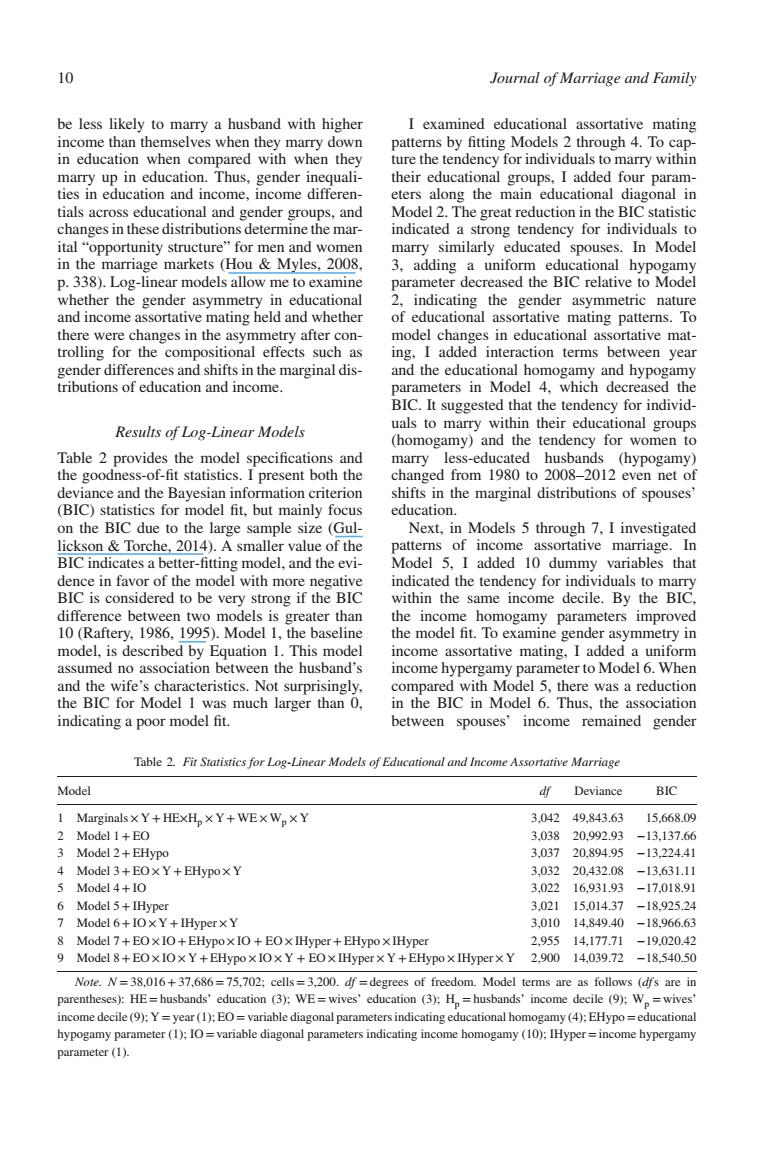
10 Journal of Marriage and Family be less likely to marry a husband with higher I examined educational assortative mating income than themselves when they marry down patterns by fitting Models 2 through 4.To cap- in education when compared with when they ture the tendency for individuals to marry within marry up in education.Thus,gender inequali- their educational groups,I added four param- ties in education and income,income differen- eters along the main educational diagonal in tials across educational and gender groups,and Model 2.The great reduction in the BIC statistic changes in these distributions determine the mar- indicated a strong tendency for individuals to ital "opportunity structure"for men and women marry similarly educated spouses.In Model in the marriage markets (Hou Myles,2008, 3,adding a uniform educational hypogamy p.338).Log-linear models allow me to examine parameter decreased the BIC relative to Model whether the gender asymmetry in educational 2. indicating the gender asymmetric nature and income assortative mating held and whether of educational assortative mating patterns.To there were changes in the asymmetry after con- model changes in educational assortative mat- trolling for the compositional effects such as ing,I added interaction terms between year gender differences and shifts in the marginal dis- and the educational homogamy and hypogamy tributions of education and income. parameters in Model 4,which decreased the BIC.It suggested that the tendency for individ- Results of Log-Linear Models uals to marry within their educational groups (homogamy)and the tendency for women to Table 2 provides the model specifications and marry less-educated husbands (hypogamy) the goodness-of-fit statistics.I present both the changed from 1980 to 2008-2012 even net of deviance and the Bayesian information criterion shifts in the marginal distributions of spouses' (BIC)statistics for model fit,but mainly focus education. on the BIC due to the large sample size (Gul- Next,in Models 5 through 7,I investigated lickson Torche,2014).A smaller value of the patterns of income assortative marriage.In BIC indicates a better-fitting model,and the evi- Model 5,I added 10 dummy variables that dence in favor of the model with more negative indicated the tendency for individuals to marry BIC is considered to be very strong if the BIC within the same income decile.By the BIC, difference between two models is greater than the income homogamy parameters improved 10 (Raftery,1986,1995).Model 1,the baseline the model fit.To examine gender asymmetry in model,is described by Equation 1.This model income assortative mating,I added a uniform assumed no association between the husband's income hypergamy parameter to Model 6.When and the wife's characteristics.Not surprisingly, compared with Model 5,there was a reduction the BIC for Model 1 was much larger than 0, in the BIC in Model 6.Thus,the association indicating a poor model fit. between spouses'income remained gender Table 2.Fit Statistics for Log-Linear Models of Educational and Income Assortative Marriage Model df Deviance BIC 1 Marginals×Y+HExH,×Y+WE×W。×Y 3.042 49.843.63 15.668.09 2 Model 1+EO 3.03820.992.93 -13.137.66 3 Model 2+EHypo 3.037 20.894.95 -13,224.41 4 Model 3+EOxY+EHypoxY 3.03220.432.08 -13.631.11 5 Model 4+IO 3.022 16.931.93 -17.018.91 6 Model 5+IHyper 3.021 15.01437 -18.925.24 7 Model 6+IOxY+IHyper xY 3.01014.849.40 -18.966.63 8 Model7+EO×IO+EHypo×IO+EO×Hyper+EHypo x IHyper 2.95514.177.71 -19.020.42 9 Model8+EOxIO×Y+EHypo×IO×Y+EOx IHyper×Y+EHypo x IHyper x Y 2.90014.039.72 -18,540.50 Note.N=38.016+37.686=75,702;cells =3,200.df =degrees of freedom.Model terms are as follows (dfs are in parentheses):HE=husbands'education (3):WE=wives'education (3):H=husbands'income decile (9):W=wives' income decile(9):Y=year(1):EO=variable diagonal parameters indicating educational homogamy(4):EHypo =educational hypogamy parameter(1):IO=variable diagonal parameters indicating income homogamy (10):IHyper=income hypergamy parameter (1).10 Journal of Marriage and Family be less likely to marry a husband with higher income than themselves when they marry down in education when compared with when they marry up in education. Thus, gender inequali￾ties in education and income, income differen￾tials across educational and gender groups, and changes in these distributions determine the mar￾ital “opportunity structure” for men and women in the marriage markets (Hou & Myles, 2008, p. 338). Log-linear models allow me to examine whether the gender asymmetry in educational and income assortative mating held and whether there were changes in the asymmetry after con￾trolling for the compositional effects such as gender differences and shifts in the marginal dis￾tributions of education and income. Results of Log-Linear Models Table 2 provides the model specifications and the goodness-of-fit statistics. I present both the deviance and the Bayesian information criterion (BIC) statistics for model fit, but mainly focus on the BIC due to the large sample size (Gul￾lickson & Torche, 2014). A smaller value of the BIC indicates a better-fitting model, and the evi￾dence in favor of the model with more negative BIC is considered to be very strong if the BIC difference between two models is greater than 10 (Raftery, 1986, 1995). Model 1, the baseline model, is described by Equation 1. This model assumed no association between the husband’s and the wife’s characteristics. Not surprisingly, the BIC for Model 1 was much larger than 0, indicating a poor model fit. I examined educational assortative mating patterns by fitting Models 2 through 4. To cap￾ture the tendency for individuals to marry within their educational groups, I added four param￾eters along the main educational diagonal in Model 2. The great reduction in the BIC statistic indicated a strong tendency for individuals to marry similarly educated spouses. In Model 3, adding a uniform educational hypogamy parameter decreased the BIC relative to Model 2, indicating the gender asymmetric nature of educational assortative mating patterns. To model changes in educational assortative mat￾ing, I added interaction terms between year and the educational homogamy and hypogamy parameters in Model 4, which decreased the BIC. It suggested that the tendency for individ￾uals to marry within their educational groups (homogamy) and the tendency for women to marry less-educated husbands (hypogamy) changed from 1980 to 2008–2012 even net of shifts in the marginal distributions of spouses’ education. Next, in Models 5 through 7, I investigated patterns of income assortative marriage. In Model 5, I added 10 dummy variables that indicated the tendency for individuals to marry within the same income decile. By the BIC, the income homogamy parameters improved the model fit. To examine gender asymmetry in income assortative mating, I added a uniform income hypergamy parameter to Model 6. When compared with Model 5, there was a reduction in the BIC in Model 6. Thus, the association between spouses’ income remained gender Table 2. Fit Statistics for Log-Linear Models of Educational and Income Assortative Marriage Model df Deviance BIC 1 Marginals × Y + HE×Hp × Y + WE × Wp × Y 3,042 49,843.63 15,668.09 2 Model 1+EO 3,038 20,992.93 −13,137.66 3 Model 2+EHypo 3,037 20,894.95 −13,224.41 4 Model 3+EO × Y +EHypo × Y 3,032 20,432.08 −13,631.11 5 Model 4+IO 3,022 16,931.93 −17,018.91 6 Model 5+IHyper 3,021 15,014.37 −18,925.24 7 Model 6+IO × Y +IHyper × Y 3,010 14,849.40 −18,966.63 8 Model 7+EO × IO +EHypo × IO + EO × IHyper+EHypo × IHyper 2,955 14,177.71 −19,020.42 9 Model 8+EO × IO × Y +EHypo × IO × Y + EO × IHyper × Y +EHypo × IHyper × Y 2,900 14,039.72 −18,540.50 Note. N =38,016+37,686=75,702; cells=3,200. df =degrees of freedom. Model terms are as follows (dfs are in parentheses): HE=husbands’ education (3); WE= wives’ education (3); Hp =husbands’ income decile (9); Wp = wives’ income decile (9); Y =year (1); EO =variable diagonal parameters indicating educational homogamy (4); EHypo=educational hypogamy parameter (1); IO =variable diagonal parameters indicating income homogamy (10); IHyper=income hypergamy parameter (1)