DENSITY ESTIMATION 595 they are sparse toward regions where the density is In this example we look at data on putts per round, higher. which is the average number of putts per round played The method of Hall and Minnotte (2002)is based for the top 175 players on the 1980 and 2001 PGA on the following result:If Hr is a smooth distribution tours.The data were taken from http://www.golfweb. function with the property fK(u)H(x-hu)du com/stats/leaders/r/1980/119 and http://www.golfweb. f(x)+0(h")and yr=H(F),where F is the dis- com/stats/leaders/r/2001/119.Interest centers on com- tribution function that corresponds to the density f= paring the results for the two years to determine if there E(f),then under smoothness conditions on f, has been any improvement. Figure 4 shows Gaussian kernel density estimates [(-A】]=+o, based on two different bandwidths for the data from 1980 and 2001 combined.The resulting 350 data Comparing this last result with(1),we see that replac- points are marked as vertical bars above the horizontal ing the data Xi by y(Xi),its so-called sharpened form, axis in Figure 4.The density estimate depicted by the produces an estimator of f(x)which is always positive dashed line in Figure 4 is based on the bandwidth ob- and for which the bias is o(h")(r=4,6,8,...)rather tained from least squares cross-validation.In this case, than the O(h2)bias of f(x). hLscv =0.054,producing an estimate with at least In practice,yr has to be estimated.Using a Taylor se- four modes,while the density estimate depicted by the solid curve in Figure 4 is based on the Sheather-Jones ries expansion on H,and plug-in estimators,Hall and plug-in bandwidth hsJ.In this case,hsJ=0.154,pro- Minnotte(2002)produced the estimators ducing an estimate with just two modes,which we see 4=1+h22(K)P below correspond to the fact that the data come from two separate years. Figure 5 shows Gaussian kernel density estimates 房=+( 2_2(K)2)f" based on two different bandwidths for the separate 2一 data sets from 1980 and 2001.The density estimates depicted by the dashed line in Figure 5 are based 2(K)2f"2(K)2(f)3 on the bandwidths obtained from least squares cross- 2f2 83 validation.In this case,hLscv =0.061 (for 2001) and 0.187 (for 1980),while the density estimates de- where denotes the identity function.Thus.the data picted by the solid curve in Figure 5 are based on the sharpened density estimator of order r is given by Sheather-Jones plug-in bandwidth hsJ.In this case, hsJ =0.121 (for 2001)and 0.158(for 1980).While A闲=2K x-(X) the two density estimates are very similar for 1980, the same is not true for 2001.The density estimate for Using a different approach,Samiuddin and El-Sayyad (1990)obtained the expression for f4.h.Note that the same bandwidth h is used for the original estimate f, all necessary derivatives and the final sharpened esti- mate.This ensures that bias terms cancel. Finally,Hall and Minnotte (2002)discovered by a0 pa Monte Carlo simulation that the optimal bandwidth for a sharpened density estimator is larger than the optimal bandwidth for a second-order kernel density estimator. g 5.REAL DATA EXAMPLE In this section we compare the performance of a 29 30 number of the bandwidth selection methods described Avera的e Number of Pults in Section 3 on a new example that involves data from FIG.4.Kernel density estimates based on LSCV (dashed curve) the PGA golf tour.A number of other examples can be and the Sheather-Jones plug-in (solid curve)for the data from 1980 found in Sheather(1992). and 2001 combined.DENSITY ESTIMATION 595 they are sparse toward regions where the density is higher. 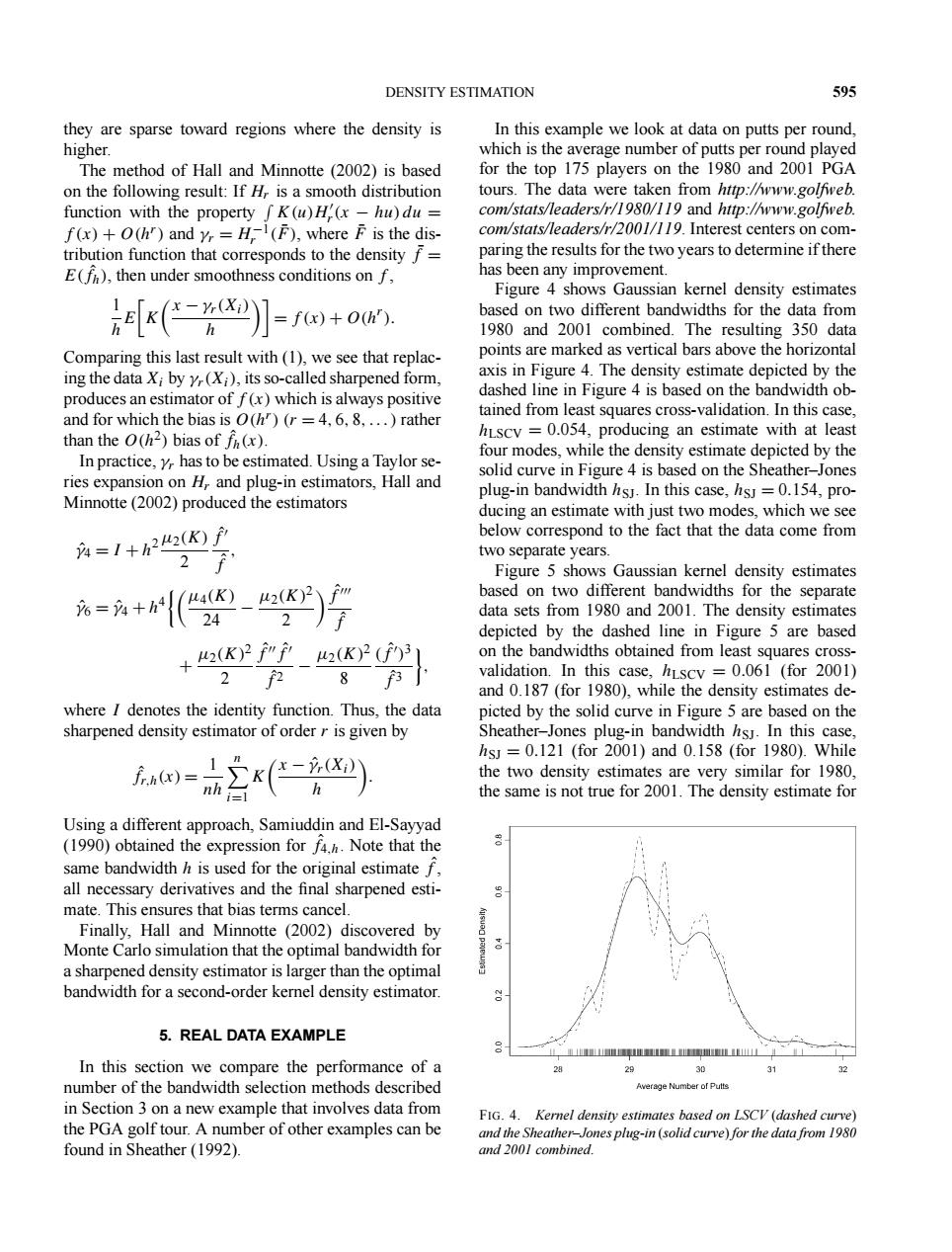The method of Hall and Minnotte (2002) is based on the following result: If Hr is a smooth distribution function with the property  K(u)H r(x − hu) du = f (x) + O(hr) and γr = H −1 r (F )¯ , where F¯ is the dis￾tribution function that corresponds to the density f¯ = E(fˆ h), then under smoothness conditions on f , 1 h E K x − γr(Xi) h  = f (x) + O(hr ). Comparing this last result with (1), we see that replac￾ing the data Xi by γr(Xi), its so-called sharpened form, produces an estimator of f (x) which is always positive and for which the bias is O(hr) (r = 4, 6, 8,...) rather than the O(h2) bias of fˆ h(x). In practice, γr has to be estimated. Using a Taylor se￾ries expansion on Hr and plug-in estimators, Hall and Minnotte (2002) produced the estimators γˆ4 = I + h2µ2(K) 2 fˆ fˆ , γˆ6 = ˆγ4 + h4 µ4(K) 24 − µ2(K)2 2 fˆ fˆ + µ2(K)2 2 fˆfˆ fˆ2 − µ2(K)2 8 (fˆ )3 fˆ3 , where I denotes the identity function. Thus, the data sharpened density estimator of order r is given by fˆ r,h(x) = 1 nh
n i=1 K x − ˆγr(Xi) h . Using a different approach, Samiuddin and El-Sayyad (1990) obtained the expression for fˆ 4,h. Note that the same bandwidth h is used for the original estimate fˆ, all necessary derivatives and the final sharpened esti￾mate. This ensures that bias terms cancel. Finally, Hall and Minnotte (2002) discovered by Monte Carlo simulation that the optimal bandwidth for a sharpened density estimator is larger than the optimal bandwidth for a second-order kernel density estimator. 5. REAL DATA EXAMPLE In this section we compare the performance of a number of the bandwidth selection methods described in Section 3 on a new example that involves data from the PGA golf tour. A number of other examples can be found in Sheather (1992). In this example we look at data on putts per round, which is the average number of putts per round played for the top 175 players on the 1980 and 2001 PGA tours. The data were taken from http://www.golfweb. com/stats/leaders/r/1980/119 and http://www.golfweb. com/stats/leaders/r/2001/119. Interest centers on com￾paring the results for the two years to determine if there has been any improvement. Figure 4 shows Gaussian kernel density estimates based on two different bandwidths for the data from 1980 and 2001 combined. The resulting 350 data points are marked as vertical bars above the horizontal axis in Figure 4. The density estimate depicted by the dashed line in Figure 4 is based on the bandwidth ob￾tained from least squares cross-validation. In this case, hLSCV = 0.054, producing an estimate with at least four modes, while the density estimate depicted by the solid curve in Figure 4 is based on the Sheather–Jones plug-in bandwidth hSJ. In this case, hSJ = 0.154, pro￾ducing an estimate with just two modes, which we see below correspond to the fact that the data come from two separate years. Figure 5 shows Gaussian kernel density estimates based on two different bandwidths for the separate data sets from 1980 and 2001. The density estimates depicted by the dashed line in Figure 5 are based on the bandwidths obtained from least squares cross￾validation. In this case, hLSCV = 0.061 (for 2001) and 0.187 (for 1980), while the density estimates de￾picted by the solid curve in Figure 5 are based on the Sheather–Jones plug-in bandwidth hSJ. In this case, hSJ = 0.121 (for 2001) and 0.158 (for 1980). While the two density estimates are very similar for 1980, the same is not true for 2001. The density estimate for FIG. 4. Kernel density estimates based on LSCV (dashed curve) and the Sheather–Jones plug-in (solid curve) for the data from 1980 and 2001 combined.