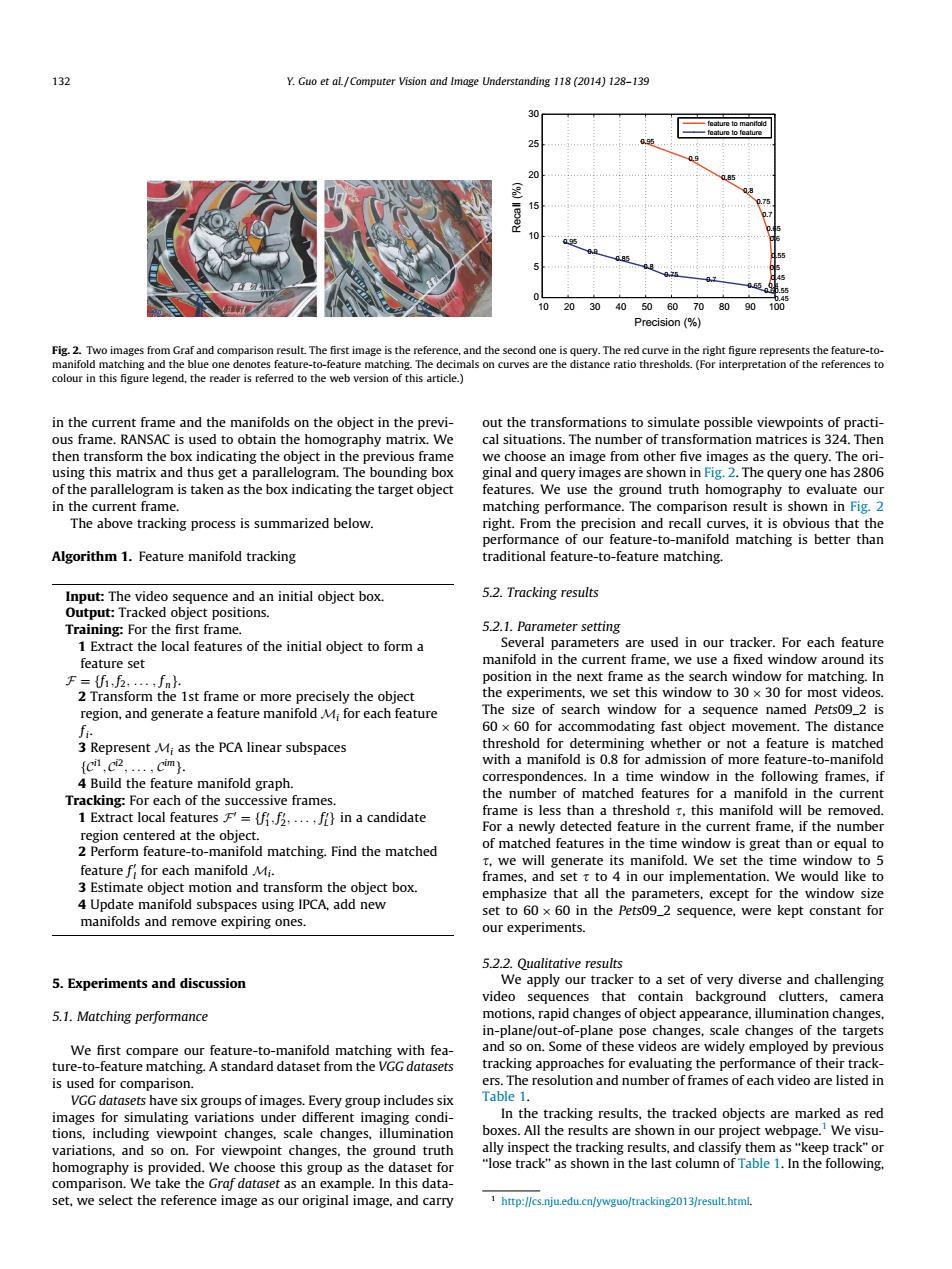
132 Y.Guo et al/Computer Vision and Image Understanding 118(2014)128-139 30 feature to feature 20 102030405060708090 100 Precision (% Fig.2.Two images from Graf and comparison result.The first image is the reference,and the second one is query.The red curve in the right figure represents the feature-to- manifold matching and the blue one denotes feature-to-feature matching.The decimals on curves are the distance ratio thresholds.(For interpretation of the references to colour in this figure legend,the reader is referred to the web version of this article.) in the current frame and the manifolds on the object in the previ- out the transformations to simulate possible viewpoints of practi- ous frame.RANSAC is used to obtain the homography matrix.We cal situations.The number of transformation matrices is 324.Then then transform the box indicating the object in the previous frame we choose an image from other five images as the query.The ori- using this matrix and thus get a parallelogram.The bounding box ginal and query images are shown in Fig.2.The query one has 2806 of the parallelogram is taken as the box indicating the target object features.We use the ground truth homography to evaluate our in the current frame. matching performance.The comparison result is shown in Fig.2 The above tracking process is summarized below. right.From the precision and recall curves,it is obvious that the performance of our feature-to-manifold matching is better than Algorithm 1.Feature manifold tracking traditional feature-to-feature matching Input:The video sequence and an initial object box. 5.2.Tracking results Output:Tracked object positions. Training:For the first frame. 5.2.1.Parameter setting 1 Extract the local features of the initial object to form a Several parameters are used in our tracker.For each feature feature set manifold in the current frame,we use a fixed window around its F=(f2.....fnh. position in the next frame as the search window for matching.In 2 Transform the 1st frame or more precisely the object the experiments,we set this window to 30 x 30 for most videos. region,and generate a feature manifold M;for each feature The size of search window for a sequence named Pets09_2 is f 60 x 60 for accommodating fast object movement.The distance 3 Represent Mi as the PCA linear subspaces threshold for determining whether or not a feature is matched (...cim) with a manifold is 0.8 for admission of more feature-to-manifold 4 Build the feature manifold graph. correspondences.In a time window in the following frames,if Tracking:For each of the successive frames. the number of matched features for a manifold in the current 1 Extract local features=ff....,f}in a candidate frame is less than a threshold t,this manifold will be removed For a newly detected feature in the current frame,if the number region centered at the object. 2 Perform feature-to-manifold matching.Find the matched of matched features in the time window is great than or equal to feature f for each manifold Mi. t,we will generate its manifold.We set the time window to 5 frames,and set t to 4 in our implementation.We would like to 3 Estimate object motion and transform the object box. emphasize that all the parameters,except for the window size 4 Update manifold subspaces using IPCA,add new set to 60x 60 in the Pets09_2 sequence,were kept constant for manifolds and remove expiring ones. our experiments. 5.2.2.Qualitative results 5.Experiments and discussion We apply our tracker to a set of very diverse and challenging video sequences that contain background clutters,camera 5.1.Matching performance motions,rapid changes of object appearance,illumination changes, in-plane/out-of-plane pose changes,scale changes of the targets We first compare our feature-to-manifold matching with fea- and so on.Some of these videos are widely employed by previous ture-to-feature matching.A standard dataset from the VGG datasets tracking approaches for evaluating the performance of their track- is used for comparison. ers.The resolution and number of frames of each video are listed in VGG datasets have six groups of images.Every group includes six Table 1. images for simulating variations under different imaging condi- In the tracking results,the tracked objects are marked as red tions,including viewpoint changes,scale changes,illumination boxes.All the results are shown in our project webpage.We visu- variations,and so on.For viewpoint changes,the ground truth ally inspect the tracking results,and classify them as "keep track"or homography is provided.We choose this group as the dataset for "lose track"as shown in the last column of Table 1.In the following. comparison.We take the Graf dataset as an example.In this data- set,we select the reference image as our original image,and carry http://cs.nju.edu.cn/ywguo/tracking2013/result.html.in the current frame and the manifolds on the object in the previ￾ous frame. RANSAC is used to obtain the homography matrix. We then transform the box indicating the object in the previous frame using this matrix and thus get a parallelogram. The bounding box of the parallelogram is taken as the box indicating the target object in the current frame. The above tracking process is summarized below. Algorithm 1. Feature manifold tracking Input: The video sequence and an initial object box. Output: Tracked object positions. Training: For the first frame. 1 Extract the local features of the initial object to form a feature set F¼ff1; f2; ... ; f ng. 2 Transform the 1st frame or more precisely the object region, and generate a feature manifold Mi for each feature fi. 3 Represent Mi as the PCA linear subspaces fCi1; Ci2; ... ; Cimg. 4 Build the feature manifold graph. Tracking: For each of the successive frames. 1 Extract local features F0 ¼ ff0 1; f0 2; ... ; f0 Lg in a candidate region centered at the object. 2 Perform feature-to-manifold matching. Find the matched feature f 0 l for each manifold Mi. 3 Estimate object motion and transform the object box. 4 Update manifold subspaces using IPCA, add new manifolds and remove expiring ones. 5. Experiments and discussion 5.1. Matching performance We first compare our feature-to-manifold matching with fea￾ture-to-feature matching. A standard dataset from the VGG datasets is used for comparison. VGG datasets have six groups of images. Every group includes six images for simulating variations under different imaging condi￾tions, including viewpoint changes, scale changes, illumination variations, and so on. For viewpoint changes, the ground truth homography is provided. We choose this group as the dataset for comparison. We take the Graf dataset as an example. In this data￾set, we select the reference image as our original image, and carry out the transformations to simulate possible viewpoints of practi￾cal situations. The number of transformation matrices is 324. Then we choose an image from other five images as the query. The ori￾ginal and query images are shown in Fig. 2. The query one has 2806 features. We use the ground truth homography to evaluate our matching performance. The comparison result is shown in Fig. 2 right. From the precision and recall curves, it is obvious that the performance of our feature-to-manifold matching is better than traditional feature-to-feature matching. 5.2. Tracking results 5.2.1. Parameter setting Several parameters are used in our tracker. For each feature manifold in the current frame, we use a fixed window around its position in the next frame as the search window for matching. In the experiments, we set this window to 30  30 for most videos. The size of search window for a sequence named Pets09_2 is 60  60 for accommodating fast object movement. The distance threshold for determining whether or not a feature is matched with a manifold is 0.8 for admission of more feature-to-manifold correspondences. In a time window in the following frames, if the number of matched features for a manifold in the current frame is less than a threshold s, this manifold will be removed. For a newly detected feature in the current frame, if the number of matched features in the time window is great than or equal to s, we will generate its manifold. We set the time window to 5 frames, and set s to 4 in our implementation. We would like to emphasize that all the parameters, except for the window size set to 60  60 in the Pets09_2 sequence, were kept constant for our experiments. 5.2.2. Qualitative results We apply our tracker to a set of very diverse and challenging video sequences that contain background clutters, camera motions, rapid changes of object appearance, illumination changes, in-plane/out-of-plane pose changes, scale changes of the targets and so on. Some of these videos are widely employed by previous tracking approaches for evaluating the performance of their track￾ers. The resolution and number of frames of each video are listed in Table 1. In the tracking results, the tracked objects are marked as red boxes. All the results are shown in our project webpage.1 We visu￾ally inspect the tracking results, and classify them as ‘‘keep track’’ or ‘‘lose track’’ as shown in the last column of Table 1. In the following, 10 20 30 40 50 60 70 80 90 100 0 5 10 15 20 25 30 0.4 0.45 0.5 0.55 0.6 0.65 0.7 0.75 0.8 0.85 0.9 0.95 0.45 0.60.55 0.65 0.7 0.75 0.8 0.85 0.9 0.95 Precision (%) Recall (%) feature to manifold feature to feature Fig. 2. Two images from Graf and comparison result. The first image is the reference, and the second one is query. The red curve in the right figure represents the feature-to￾manifold matching and the blue one denotes feature-to-feature matching. The decimals on curves are the distance ratio thresholds. (For interpretation of the references to colour in this figure legend, the reader is referred to the web version of this article.) 1 http://cs.nju.edu.cn/ywguo/tracking2013/result.html. 132 Y. Guo et al. / Computer Vision and Image Understanding 118 (2014) 128–139