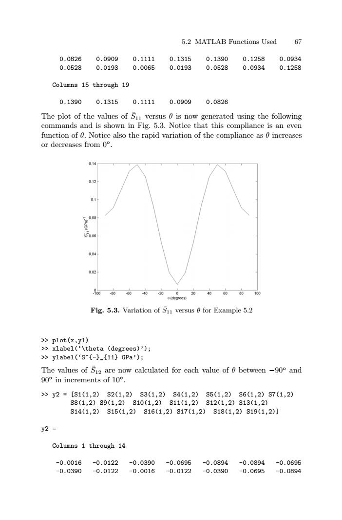
5.2 MATLAB Functions Used 67 0.0826 0.0909 0.1111 0.1315 0.1390 0.1258 0.0934 0.0528 0.0193 0.0065 0.0193 0.0528 0.0934 0.1258 Columns 15 through 19 0.1390 0.13150.1111 0.09090.0826 The plot of the values of Su versus is now generated using the following commands and is shown in Fig.5.3.Notice that this compliance is an even function of 0.Notice also the rapid variation of the compliance as 0 increases or decreases from0°. 0.14 005 0.0时 0.04 0.02 80 60 4020020406060100 e(degrees) Fig.5.3.Variation of S11 versus 0 for Example 5.2 >plot(x,y1) >xlabel('\theta (degrees)'); >>y1abe1(‘s{-J-{11}GPa'); The values of 512 are now calculated for each value of between-90 and 90°in increments of10°. >>y2=[S1(1,2)S2(1,2)S3(1,2)S4(1,2)S5(1,2)S6(1,2)S7(1,2) S8(1,2)S9(1,2)S10(1,2)S11(1,2)S12(1,2)S13(1,2) S14(1,2)S15(1,2)S16(1,2)S17(1,2)S18(1,2)S19(1,2)] y2= Columns 1 through 14 -0.0016 -0.0122 -0.0390 -0.0695 -0.0894 -0.0894 -0.0695 -0.0390 -0.0122 -0.0016 -0.0122 -0.0390 -0.0695 -0.08945.2 MATLAB Functions Used 67 0.0826 0.0909 0.1111 0.1315 0.1390 0.1258 0.0934 0.0528 0.0193 0.0065 0.0193 0.0528 0.0934 0.1258 Columns 15 through 19 0.1390 0.1315 0.1111 0.0909 0.0826 The plot of the values of S¯11 versus θ is now generated using the following commands and is shown in Fig. 5.3. Notice that this compliance is an even function of θ. Notice also the rapid variation of the compliance as θ increases or decreases from 0◦. Fig. 5.3. Variation of S¯11 versus θ for Example 5.2 >> plot(x,y1) >> xlabel(‘\theta (degrees)’); >> ylabel(‘S^{-}_{11} GPa’); The values of S¯12 are now calculated for each value of θ between −90◦ and 90◦ in increments of 10◦. >> y2 = [S1(1,2) S2(1,2) S3(1,2) S4(1,2) S5(1,2) S6(1,2) S7(1,2) S8(1,2) S9(1,2) S10(1,2) S11(1,2) S12(1,2) S13(1,2) S14(1,2) S15(1,2) S16(1,2) S17(1,2) S18(1,2) S19(1,2)] y2 = Columns 1 through 14 -0.0016 -0.0122 -0.0390 -0.0695 -0.0894 -0.0894 -0.0695 -0.0390 -0.0122 -0.0016 -0.0122 -0.0390 -0.0695 -0.0894