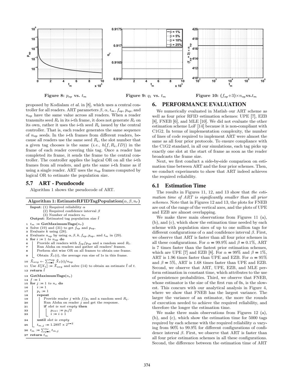
0.9175 420 -B=1% B=5% 10 -B=10% 418 0.917 B=25 10 416 .414 0.9165 0 412 0.910 410 10 10 10 104 10 x10 x10 Figure 8:Pop vs.tm Figure 9:q1 vs.tm Figure 10:(fop+3)xnopvs.tm proposed by Kodialam et al.in [8],which uses a central con- 6. PERFORMANCE EVALUATION troller for all readers.ART parameters B,a,tm,fop,Pop,and We numerically evaluated in Matlab our ART scheme as nop have the same value across all readers.When a reader well as four prior RFID estimation schemes:UPE 7.EZB transmits seed Ri in its i-th frame,it does not generate Ri on 8,FNEB 6],and MLE 10.We did not evaluate the other its own,rather it uses the i-th seed Ri issued by the central estimation scheme LoF [14]because it is non-compliant with controller.That is,each reader generates the same sequence C1G2.In terms of implementation complexity,the number of nop seeds.In the i-th frames from different readers,be- of lines of code required to implement ART were almost the cause all readers use the same seed Ri,the slot number that same as all four prior protocols.To ensure compliance with a given tag chooses is the same (i.e.,h(f,Ri,ID))in the the C1G2 standard,in all our simulations,each tag picks up frame of each reader covering this tag.Once a reader has exactly one slot at the start of frame as soon as the reader completed its frame,it sends the frame to the central con- broadcasts the frame size. troller.The controller applies the logical OR on all the i-th Next,we first conduct a side-by-side comparison on esti- frames from all readers,and gets the same i-th frame as if mation time between ART and the four prior schemes.Then. using a single reader.ART uses the nop frames computed by we conduct experiments to show that ART indeed achieves logical OR to estimate the population size. the required reliability 5.7 ART-Pseudocode 6.1 Estimation Time Algorithm 1 shows the pseudocode of ART The results in Figures 11,12,and 13 show that the esti- mation time of ART is significantly smaller than all prior Algorithm 1:EstimateRFIDTagPopulation(a,B,nr) schemes.Note that in Figures 12 and 13,the plots for FNEB Input:(1)Required reliability a are out of the range of the vertical axes,and the plots of UPE (2)Required confidence interval B and EZB are almost overlapping. (3)Number of readers nr Output:Estimated tag population size f We make three main observations from Figures 11 (a) 1tm :=GetMaximumTags(nr) (b),and (c),which show the estimation time needed by each 2 Solve (19)and (31)to get fop and pop. scheme with population sizes of up to one million tags for 3 Evaluate k using (28). different configurations of a and confidence interval B.First. 4 Evaluate nop by using a,B,k,fop:Pop:and tm in (29). s for i:=1 to nop do we observe that ART is faster than all four prior schemes in Provide all readers with fop/pop and a random seed Ri. all these configurations.For a=99.9%and B=0.1%,ART 7 Run Aloha on readers and gather all readers'frames. is 7 times faster than the fastest prior estimation schemes Perform slot wise OR on all frames to obtain one frame. which are UPE 7 and EZB 8.For a =99%and B=1% Obtain X1(i),the average run size of 1s in this frame. ART is 1.96 times faster than UPE and EZB.For a=95% 10文avg←∑2文1()/mop and B=5%.ART is 1.68 times faster than UPE and EZB 11 Use E[X]:=and solve (14)to obtain an estimate i of t. Second.we observe that ART,UPE.EZB,and MLE per- 12 return t form estimation in constant time,which attributes to the use 13 GetMaximumTags(n,) 14 f:=1 of persistence probabilities.Third,we observe that FNEB 16 for j:=1 to nr do whose estimator is the size of the first run of 0s,is the slow- 16 i=1 est.This concurs with our analytical analysis in Figure 4. 17 P=1 where we show that FNEB has the largest variance.The 18 repeat Provide reader j with f/p and a random seed Ri larger the variance of an estimator,the more the rounds 0 Run Aloha on reader j and get the response. of execution needed to achieve the required reliability,and 21 if slot is not empty then therefore the longer the estimation time. p4+1=p4/2 28 i:=i+1 We make three main observations from Figures 12(a), 24 until slot is empty (b),and (c),which show the estimation time for 5000 tags 26 tm,=1.2897×2-2 required by each scheme with the required reliability a vary- 26 tm=∑r1tmd ing from 90%to 99.9%for different configurations of confi- 27 return tm dence interval B.First,we observe that ART is faster than all four prior estimation schemes in all these configurations Second,the difference between the estimation time of ART 3740 2 4 6 8 10 x 105 10−4 10−3 10−2 10−1 100 t m pop Figure 8: pop vs. tm 2 4 6 8 10 x 105 0.916 0.9165 0.917 0.9175 t m q1 β = 1% β = 5% β = 10% β = 25% Figure 9: q1 vs. tm 102 103 104 105 106 410 412 414 416 418 420 t m (fop+ 3) × nop Figure 10: (fop+3)×nopvs.tm proposed by Kodialam et al. in [8], which uses a central con￾troller for all readers. ART parameters β, α, tm, fop, pop, and nop have the same value across all readers. When a reader transmits seed Ri in its i-th frame, it does not generate Ri on its own, rather it uses the i-th seed Ri issued by the central controller. That is, each reader generates the same sequence of nop seeds. In the i-th frames from different readers, be￾cause all readers use the same seed Ri, the slot number that a given tag chooses is the same (i.e., h(f,Ri,ID)) in the frame of each reader covering this tag. Once a reader has completed its frame, it sends the frame to the central con￾troller. The controller applies the logical OR on all the i-th frames from all readers, and gets the same i-th frame as if using a single reader. ART uses the nop frames computed by logical OR to estimate the population size. 5.7 ART - Pseudocode Algorithm 1 shows the pseudocode of ART. Algorithm 1: EstimateRFIDTagPopulation(α, β, nr) Input: (1) Required reliability α (2) Required confidence interval β (3) Number of readers nr Output: Estimated tag population size t ˜ 1 tm := GetMaximumTags(nr) 2 Solve (19) and (31) to get fop and pop. 3 Evaluate k using (28). 4 Evaluate nop by using α, β, k, fop, pop, and tm in (29). 5 for i := 1 to nop do 6 Provide all readers with fop/pop and a random seed Ri. 7 Run Aloha on readers and gather all readers’ frames. 8 Perform slot wise OR on all frames to obtain one frame. 9 Obtain X˜1(i), the average run size of 1s in this frame. 10 X˜avg ← nop i=1 X˜1(i)/nop 11 Use E[X1] := X˜avg and solve (14) to obtain an estimate t ˜ of t. 12 return t ˜ 13 GetMaximumTags(nr) 14 f := 1 15 for j := 1 to nr do 16 i := 1 17 pi := 1 18 repeat 19 Provide reader j with f/pi and a random seed Ri. 20 Run Aloha on reader j and get the response. 21 if slot is not empty then 22 pi+1 := pi/2 23 i := i + 1 24 until slot is empty 25 tm,j := 1.2897 × 2i−2 26 tm := nr j=1 tm,j 27 return tm 6. PERFORMANCE EVALUATION We numerically evaluated in Matlab our ART scheme as well as four prior RFID estimation schemes: UPE [7], EZB [8], FNEB [6], and MLE [10]. We did not evaluate the other estimation scheme LoF [14] because it is non-compliant with C1G2. In terms of implementation complexity, the number of lines of code required to implement ART were almost the same as all four prior protocols. To ensure compliance with the C1G2 standard, in all our simulations, each tag picks up exactly one slot at the start of frame as soon as the reader broadcasts the frame size. Next, we first conduct a side-by-side comparison on esti￾mation time between ART and the four prior schemes. Then, we conduct experiments to show that ART indeed achieves the required reliability. 6.1 Estimation Time The results in Figures 11, 12, and 13 show that the esti￾mation time of ART is significantly smaller than all prior schemes. Note that in Figures 12 and 13, the plots for FNEB are out of the range of the vertical axes, and the plots of UPE and EZB are almost overlapping. We make three main observations from Figures 11 (a), (b), and (c), which show the estimation time needed by each scheme with population sizes of up to one million tags for different configurations of α and confidence interval β. First, we observe that ART is faster than all four prior schemes in all these configurations. For α = 99.9% and β = 0.1%, ART is 7 times faster than the fastest prior estimation schemes, which are UPE [7] and EZB [8]. For α = 99% and β = 1%, ART is 1.96 times faster than UPE and EZB. For α = 95% and β = 5%, ART is 1.68 times faster than UPE and EZB. Second, we observe that ART, UPE, EZB, and MLE per￾form estimation in constant time, which attributes to the use of persistence probabilities. Third, we observe that FNEB, whose estimator is the size of the first run of 0s, is the slow￾est. This concurs with our analytical analysis in Figure 4, where we show that FNEB has the largest variance. The larger the variance of an estimator, the more the rounds of execution needed to achieve the required reliability, and therefore the longer the estimation time. We make three main observations from Figures 12 (a), (b), and (c), which show the estimation time for 5000 tags required by each scheme with the required reliability α vary￾ing from 90% to 99.9% for different configurations of confi- dence interval β. First, we observe that ART is faster than all four prior estimation schemes in all these configurations. Second, the difference between the estimation time of ART 374