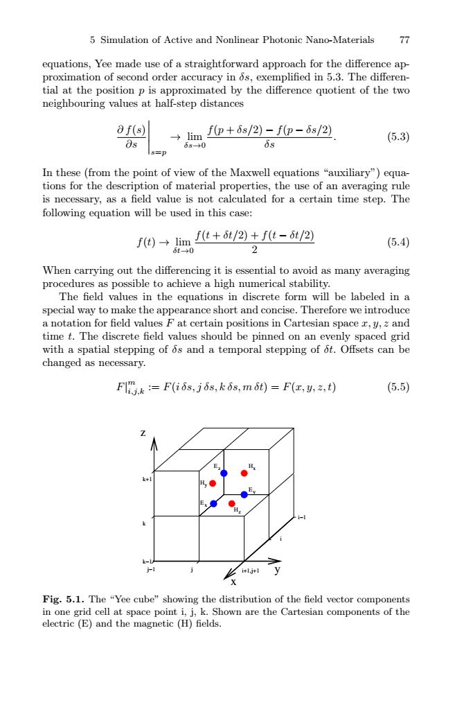
5 Simulation of Active and Nonlinear Photonic Nano-Materials 77 equations,Yee made use of a straightforward approach for the difference ap- proximation of second order accuracy in 6s,exemplified in 5.3.The differen- tial at the position p is approximated by the difference quotient of the two neighbouring values at half-step distances 0f(s) lim f(p+s/2)-fp-6s/2) (5.3) os 68+0 0s 8=p In these(from the point of view of the Maxwell equations "auxiliary")equa- tions for the description of material properties,the use of an averaging rule is necessary,as a field value is not calculated for a certain time step.The following equation will be used in this case: f(e)→1im f(t+t/2)+f(t-t/2) (5.4) 6t→0 2 When carrying out the differencing it is essential to avoid as many averaging procedures as possible to achieve a high numerical stability. The field values in the equations in discrete form will be labeled in a special way to make the appearance short and concise.Therefore we introduce a notation for field values F at certain positions in Cartesian space r,y,z and time t.The discrete field values should be pinned on an evenly spaced grid with a spatial stepping of os and a temporal stepping of ot.Offsets can be changed as necessary. F昭k=F(i6s,j6s,ki,m60）=F(z,2,) (5.5) + ijy X Fig.5.1.The "Yee cube"showing the distribution of the field vector components in one grid cell at space point i,j,k.Shown are the Cartesian components of the electric (E)and the magnetic (H)fields.5 Simulation of Active and Nonlinear Photonic Nano-Materials 77 equations, Yee made use of a straightforward approach for the difference ap￾proximation of second order accuracy in δs, exemplified in 5.3. The differen￾tial at the position p is approximated by the difference quotient of the two neighbouring values at half-step distances ∂ f(s) ∂s      s=p → lim δs→0 f(p + δs/2) − f(p − δs/2) δs . (5.3) In these (from the point of view of the Maxwell equations “auxiliary”) equa￾tions for the description of material properties, the use of an averaging rule is necessary, as a field value is not calculated for a certain time step. The following equation will be used in this case: f(t) → lim δt→0 f(t + δt/2) + f(t − δt/2) 2 (5.4) When carrying out the differencing it is essential to avoid as many averaging procedures as possible to achieve a high numerical stability. The field values in the equations in discrete form will be labeled in a special way to make the appearance short and concise. Therefore we introduce a notation for field values F at certain positions in Cartesian space x, y, z and time t. The discrete field values should be pinned on an evenly spaced grid with a spatial stepping of δs and a temporal stepping of δt. Offsets can be changed as necessary. F| m i,j,k := F(i δs, j δs, k δs, m δt) = F(x, y, z, t) (5.5) j−1 j i+1,j+1 i k+1 k k−1 x y z E H z y H E H Ex z y x i−1 Fig. 5.1. The “Yee cube” showing the distribution of the field vector components in one grid cell at space point i, j, k. Shown are the Cartesian components of the electric (E) and the magnetic (H) fields